Student t 分配百分位點（逆 t / 分位數）計算器

輸入計算

累積機率 P 須嚴格介於 0 與 1 之間的機率（例如 0.975）。

尾端類型 Lower (P = area to the LEFT of t) Upper (P = area to the RIGHT of t)

自由度（nu） 任何正數皆可，通常為正整數。

結果

百分位點 t

2.228139

滿足 F(t) = 左尾機率的分位數

實際採用的左尾機率	0.975
結果解讀	F(t) = P(T ≤ t) = 0.975

這個計算器的用途

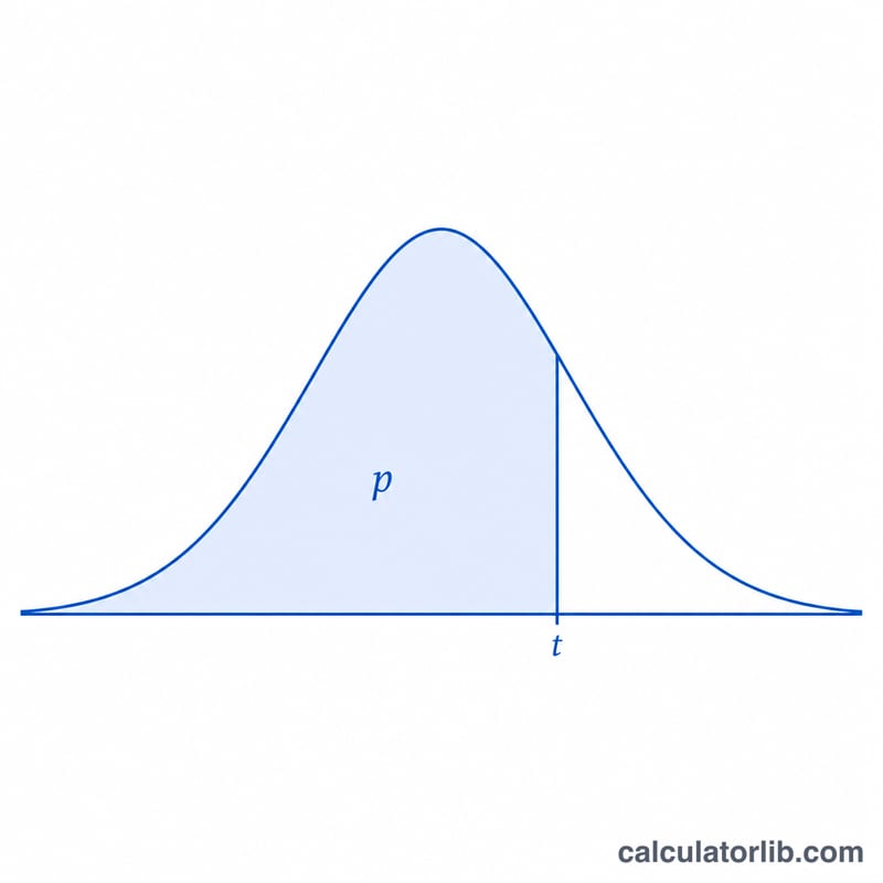
本工具用來計算 Student t 分配的百分位點（也稱為分位數、臨界值或逆累積分配函數）。只要輸入累積機率 P 與自由度 nu，工具就會回傳一個 t 值，使得 t 密度曲線到 t 為止所涵蓋的面積，恰好等於您所設定的機率。這正是 t 分配累積分配函數（CDF）的反函數，對應試算表中的 t.inv 函數。t 分配屬於通用的純數學，全世界的計算結果完全相同。

The percentage point t is the value where the cumulative area under the t-distribution curve equals p.

使用方法

輸入累積機率 P（須嚴格介於 0 與 1 之間），接著選擇 P 代表的是左尾面積（t 左側）還是右尾面積（t 右側），最後輸入自由度。計算器內部一律會轉換成左尾機率：若選左尾，直接使用 P；若選右尾，則改用 \(1 - P\)，再據此求解 t。

公式說明

自由度為 nu 的 Student t 分配，其 CDF 可用正規化不完全 Beta 函數 I 來表示。當 \(t \ge 0\) 時， $$F(t) = 1 - \tfrac{1}{2}\,I_{x}\!\left(\tfrac{\nu}{2},\tfrac{1}{2}\right),\quad x=\frac{\nu}{\nu+t^{2}}$$ 當 \(t < 0\) 時，則使用對稱式 $$F(t) = \tfrac{1}{2}\,I_{x}\!\left(\tfrac{\nu}{2},\tfrac{1}{2}\right)$$ 不完全 Beta 函數的計算，採用 Lanczos 近似法處理 gamma 函數，並搭配標準的連分數演算法。由於 F 為嚴格遞增函數，因此可透過穩健的二分法求得其反函數： $$t = F^{-1}\!\left(\text{P};\ \nu\right)$$

Advertisement

The t-distribution has heavier tails than the normal curve, narrowing toward it as degrees of freedom grow.

實例演算

當 \(P = 0.975\)、左尾、自由度 \(\nu = 10\) 時，計算器會回傳 $$t \approx 2.228139$$ —— 也就是 t 分配表中常見的雙尾 95%（單尾 97.5%）臨界值。若改以 \(P = 0.025\) 搭配右尾，也會得到相同結果，因為右尾 2.5% 的面積等同於左尾 97.5% 的面積。

常見問題

如果輸入 \(P = 0\) 或 \(P = 1\) 會怎樣？此時百分位點沒有定義，會發散至負無限大或正無限大，計算器會回報錯誤。

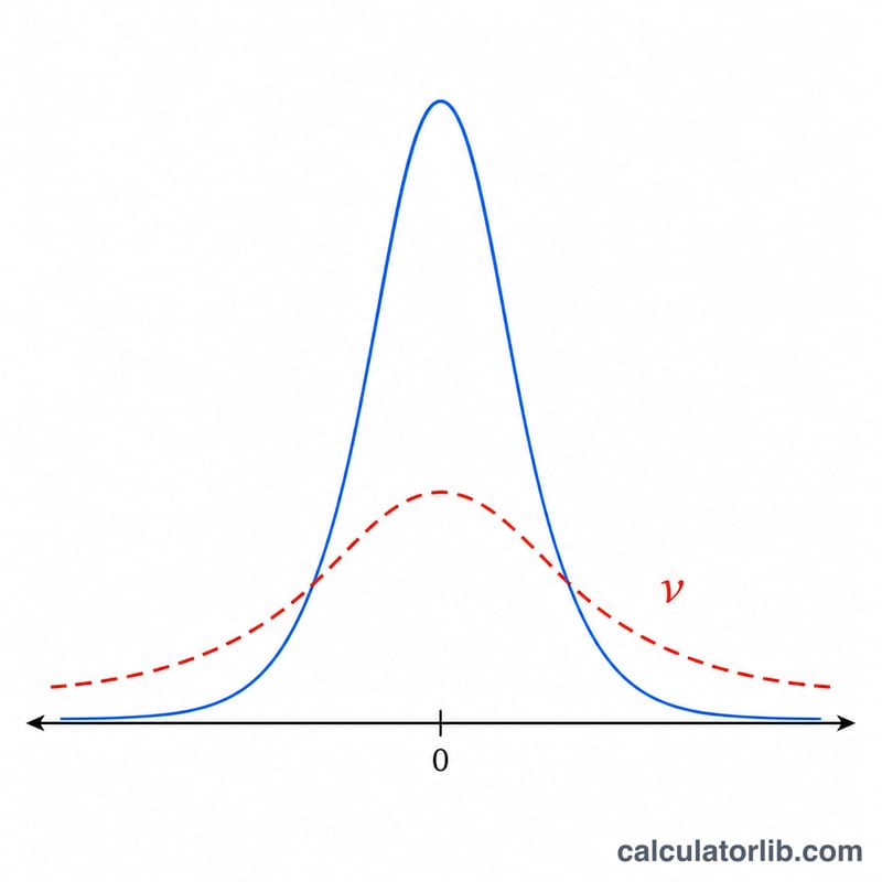
當自由度變得很大時會發生什麼？t 分配會逐漸趨近標準常態分配，因此當 nu 非常大時，分位數會接近常態分配的分位數（例如 \(P = 0.975\) 約為 \(1.95996\)）。

nu 可以是非整數嗎？可以。任何大於 0 的 nu 都能接受，包含小數值。