What is the Pareto Distribution Percentile Calculator?
This tool computes the percentile, also called the quantile, of a Pareto Type I distribution. Given a target cumulative probability and the distribution's two parameters — the scale parameter a (the minimum value x_m) and the shape parameter b (alpha, the tail index) — it returns the value x at which the distribution reaches that probability. The Pareto distribution is widely used to model wealth, income, city sizes, file sizes, and other heavy-tailed phenomena that follow the "80/20" pattern.
How to use it
First choose the cumulative mode. Select "Lower cumulative P" if your probability is the lower-tail CDF value \(P = \Pr(X \le x)\), or "Upper cumulative Q" if it is the upper-tail survival value \(Q = \Pr(X > x)\). Enter the cumulative probability between 0 and 1, then the scale parameter a (must be greater than 0) and the shape parameter b (must be greater than 0). The calculator normalizes your input to a lower-tail probability and inverts the CDF.
The formula explained
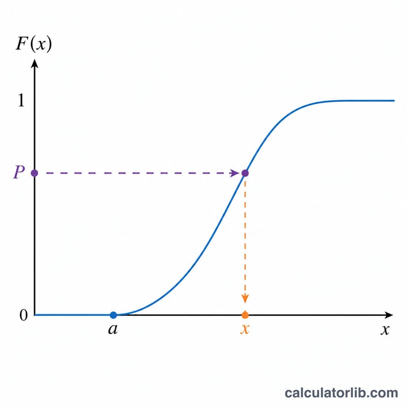
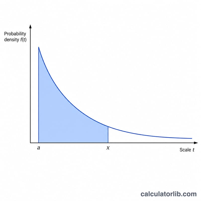
The Pareto Type I CDF for \(x \ge a\) is \(P(x) = 1 - (a/x)^b\). Solving for x gives $$x = \text{a} \cdot \left(1 - \text{P}\right)^{-1/\text{b}}.$$ When you supply an upper-tail probability Q, note that \(1 - P = Q\), so the formula becomes $$x = \text{a} \cdot \left(\text{Q}\right)^{-1/\text{b}}.$$ Because \(a > 0\) and \(0 \le 1 - P \le 1\) with \(b > 0\), the result always satisfies \(x \ge a\), landing within the distribution's support.
Worked example
Take the upper-tail case with \(Q = 0.1\), \(a = 2\), and \(b = 3\). Then $$x = 2 \cdot (0.1)^{-1/3} = 2 \cdot 10^{1/3} = 2 \cdot 2.15443 = 4.30887.$$ Checking: \(Q(x) = (2 / 4.30887)^3 \approx 0.1\), confirming the result. For the standard Pareto with \(a = 1\), \(b = 1\) and \(P = 0.5\), the median is $$x = 1 / (1 - 0.5) = 2.$$
FAQ
What happens at P = 1 (or Q = 0)? The quantile is unbounded (infinity), because the Pareto distribution has an infinitely long right tail. The calculator flags this rather than dividing by zero.
What does the result mean when P = 0? The quantile equals a, the minimum value and left endpoint of the support.
What is the difference between scale and shape? The scale a sets the minimum possible value, while the shape b controls how heavy the tail is — smaller b means a heavier tail and larger extreme values.


