

What is the Generalized Pareto Distribution percentile?
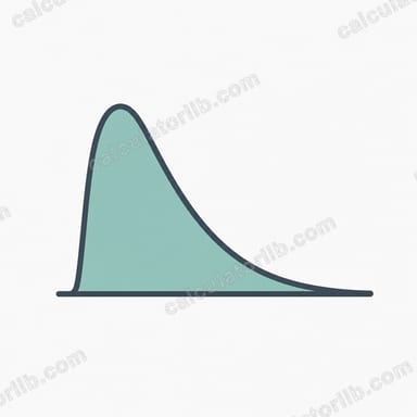
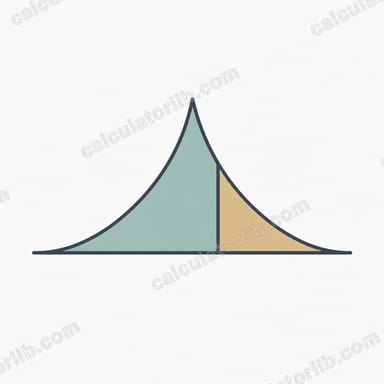
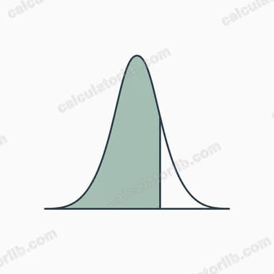
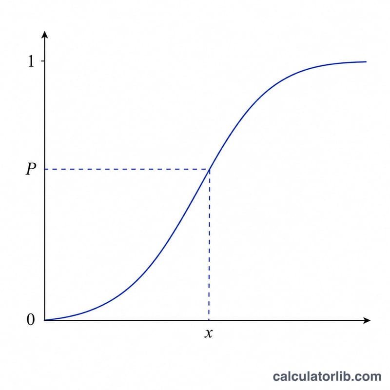
The Generalized Pareto Distribution (GPD) is a continuous probability distribution widely used in extreme-value statistics to model the tail behaviour of data — exceedances over a high threshold. Its percentile (also called the quantile or percent point) is the value x for which the cumulative probability F(x) equals a chosen probability P. This calculator evaluates the inverse cumulative distribution function (inverse CDF) given the three standard parameters: location mu, scale sigma, and shape xi. It is a pure statistical function and is not specific to any country or jurisdiction.
How to use the calculator
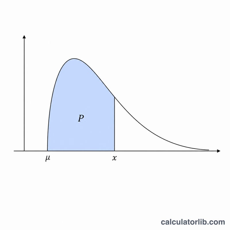
First choose the cumulative mode. Select "Lower cumulative P" when your probability is \(P = \Pr(X \le x)\). Select "Upper cumulative Q" when your probability is the survival probability \(Q = \Pr(X > x)\); the tool internally converts it with \(P = 1 - Q\). Then enter the cumulative probability (between 0 and 1), the location mu, the scale sigma (must be greater than 0), and the shape xi. The result is the percentile x at that probability point.
The formula explained
The GPD CDF is $$F(x) = 1 - \left(1 + \frac{\xi\,(x - \mu)}{\sigma}\right)^{-1/\xi}$$ for \(\xi \ne 0\), and $$F(x) = 1 - \exp\left(-\frac{x - \mu}{\sigma}\right)$$ when \(\xi = 0\). Inverting for x given a lower cumulative probability P gives $$x = \mu + \frac{\sigma}{\xi}\left[(1 - P)^{-\xi} - 1\right]$$ when \(\xi \ne 0\), and $$x = \mu - \sigma\,\ln(1 - P)$$ when \(\xi = 0\). Because dividing by xi fails at zero, any \(|\xi| < 10^{-12}\) is treated as the exponential case.
Worked example
With mode = lower, P = 0.9, mu = 0, sigma = 1, xi = 0.5: $$x = \frac{1}{0.5}\cdot\left[(1 - 0.9)^{-0.5} - 1\right] = 2\cdot\left[0.1^{-0.5} - 1\right] = 2\cdot\left[3.1622777 - 1\right] = 4.3245553.$$
FAQ
What happens when xi = 0? The GPD collapses to a shifted exponential distribution, and the quantile uses the logarithmic formula above.
Is the upper support always infinite? No. If \(\xi < 0\) the support is bounded above at \(x = \mu - \sigma/\xi\); at \(P = 1\) the calculator returns this finite endpoint. If \(\xi \ge 0\) the upper tail is unbounded and \(P = 1\) yields positive infinity.
Why must sigma be positive? The scale parameter sigma sets the spread of the distribution; a non-positive sigma makes the distribution undefined.