What is Amdahl's Law?
Amdahl's Law, formulated by computer architect Gene Amdahl in 1967, predicts the maximum theoretical speedup of a task when only part of it can be parallelized. It is a cornerstone of parallel computing and helps engineers set realistic expectations before investing in more processors, cores, or threads.
How to use this calculator
Enter two values: the parallel portion (p) — the fraction of the program (between 0 and 1) that can be run in parallel — and the speedup factor (s), typically the number of processors or cores applied to that parallel part. The calculator returns the overall speedup, the theoretical maximum speedup, and the parallel efficiency.
The formula explained
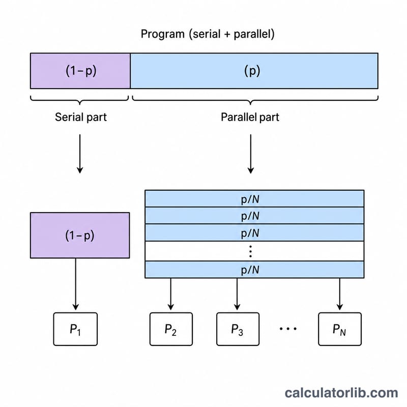
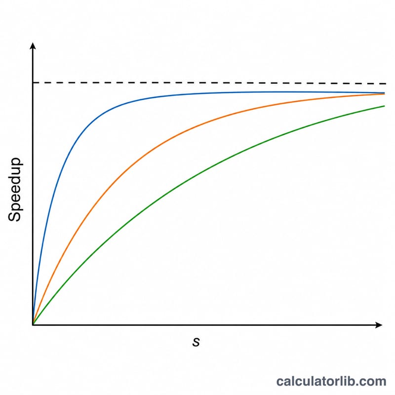
The equation is $$\text{Speedup} = \dfrac{1}{(1 - p) + \dfrac{p}{s}}$$ The term \((1 - p)\) is the serial fraction that cannot be sped up at all. As \(s\) grows very large, \(p/s\) approaches zero, so speedup is capped at \(\dfrac{1}{1 - p}\). This is why a program that is 90% parallel can never run more than 10× faster, no matter how many processors you add.
Worked example
Suppose 90% of a program is parallelizable (\(p = 0.9\)) and you use 4 processors (\(s = 4\)). Then denominator $$= (1 - 0.9) + \dfrac{0.9}{4} = 0.1 + 0.225 = 0.325.$$ Speedup $$= \dfrac{1}{0.325} \approx 3.08\times.$$ The maximum possible speedup is \(\dfrac{1}{0.1} = 10\times\), and efficiency is \(3.08 / 4 \approx 76.9\%\).
Interpreting Your Result
Overall speedup is what you actually get with the processor count \(s\) you entered — for example, a result of 4.71× means the parallelized program runs about 4.71 times faster than the single-processor version. Maximum speedup, \(1/(1-p)\), is the absolute ceiling you would approach with infinitely many processors. The gap between the two tells you how much room is left: if your overall speedup is already close to the maximum, adding hardware will barely help.
Efficiency answers "how well am I using the processors I'm paying for?" An efficiency near 100% means each processor is contributing nearly a full unit of speedup — an excellent use of resources. Low efficiency (say, under 30%) means most processors are idling or waiting on the serial portion, so you are paying for hardware that does little useful work.
The serial fraction \(1-p\) is the decisive limit. Even a small serial fraction caps performance hard: at \(p=0.95\) the ceiling is only 20×, so beyond roughly 16–32 processors each new processor adds almost nothing. A practical rule of thumb is to stop adding processors once efficiency drops below your acceptable threshold (often 50–70% for cost-sensitive work), because past that point you are spending money for vanishing gains. To push the ceiling higher, you must reduce the serial fraction itself — algorithmic changes that increase \(p\) usually pay off far more than simply adding cores.
Key Terms & Variables
- Parallel fraction (\(p\)) — the proportion of the program's work that can be executed in parallel, expressed as a decimal between 0 and 1. A value of 0.9 means 90% of the workload can be split across processors.
- Serial fraction (\(1-p\)) — the portion that must run sequentially on a single processor and cannot be sped up by parallelization. This fraction sets the hard upper limit on overall speedup.
- Speedup of the parallel part (\(s\)) — the factor by which the parallelizable portion is accelerated, typically equal to the number of processors or cores applied to it.
- Overall speedup — the ratio of single-processor execution time to parallel execution time, \(1/\big((1-p)+p/s\big)\). This is the real-world performance gain.
- Maximum speedup — the theoretical limit \(1/(1-p)\) reached as \(s\) grows without bound, determined solely by the serial fraction.
- Parallel efficiency — overall speedup divided by the number of processors, \(\text{Speedup}/s\), expressed as a percentage; it measures how effectively each processor is utilized.
FAQ
Why does adding processors give diminishing returns? Because the serial portion becomes the bottleneck. Once it dominates, extra processors barely help.
What is parallel efficiency? It is speedup divided by the number of processors, expressed as a percentage — how effectively each processor is being used.
How does this differ from Gustafson's Law? Amdahl's Law assumes a fixed problem size; Gustafson's Law assumes the problem scales with the number of processors, giving more optimistic results.