
What is Amdahl's Law?
Amdahl's Law, formulated by computer architect Gene Amdahl in 1967, predicts the maximum theoretical speedup of a task when only part of it can be parallelized. It is a cornerstone of parallel computing and helps engineers decide whether adding more processors, cores, or threads is worth the effort. The key insight is that the serial (non-parallelizable) portion of a program ultimately limits how fast it can run, no matter how many resources you throw at the parallel portion.
How to use this calculator
Enter two values: the parallel portion of your program as a percentage (the fraction of work that can be split across processors), and the speedup of the parallel part, which is usually the number of processors or cores executing it. The calculator returns the overall speedup, the maximum theoretical speedup if the parallel speedup were infinite, and the parallel efficiency.
The formula explained
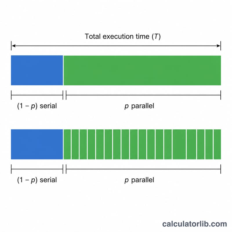
The equation is $$\text{Speedup} = \dfrac{1}{(1 - p) + \dfrac{p}{s}}$$ where \(p\) is the parallel fraction (between 0 and 1) and \(s\) is the speedup applied to that fraction. The term \((1 - p)\) is the serial part that cannot be accelerated. As \(s\) approaches infinity, the speedup converges to \(\dfrac{1}{1 - p}\), the hard ceiling imposed by the serial portion.
Worked example
Suppose 90% of a program is parallelizable (\(p = 0.9\)) and you run it on 8 processors (\(s = 8\)). Then the denominator is $$(1 - 0.9) + \frac{0.9}{8} = 0.1 + 0.1125 = 0.2125,$$ giving a speedup of \(\dfrac{1}{0.2125} \approx 4.71\times\). Even with infinite processors the maximum speedup is only \(\dfrac{1}{0.1} = 10\times\), illustrating how the 10% serial portion caps performance.
Interpreting Your Result
The speedup value tells you how many times faster the program runs with \(s\) processors compared to running on a single processor. A speedup of 4× means the parallelized workload finishes in one-quarter of the original time. Because Amdahl's Law assumes a fixed problem size, the speedup is bounded by the serial fraction \(1-p\) that cannot be sped up.
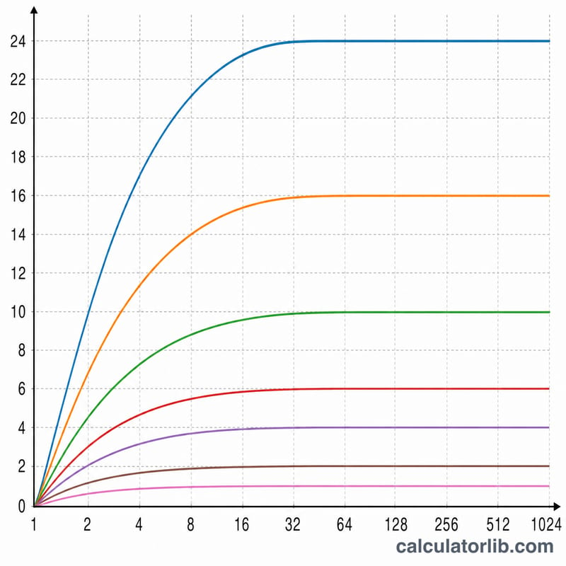
The infinite-processor ceiling, \(1/(1-p)\), is the maximum speedup achievable with unlimited hardware. For example, if 95% of the work is parallel, the ceiling is \(1/(1-0.95) = 20\times\); even a million cores cannot beat 20×. This is the single most important number for planning: it sets the upper limit on any investment in additional processors.
Parallel efficiency measures how well processors are utilized and is defined as the speedup divided by the number of processors, \(\text{efficiency} = \text{Speedup}/s\). An efficiency of 1.0 (100%) is perfect linear scaling; in practice it falls as you add cores. For instance, 90% parallel code on 8 cores gives a speedup of 4.71×, so efficiency is \(4.71/8 \approx 59\%\) — each added core does progressively less useful work.
Adding processors stops being worthwhile when the marginal speedup per additional core becomes small relative to its cost and when efficiency drops below an acceptable threshold (often 50–70% in practice). Once the speedup approaches its ceiling, further hardware yields almost nothing. To raise the ceiling itself you must reduce the serial fraction — by parallelizing more of the algorithm or reducing synchronization and I/O — rather than buying more cores. Note also that Amdahl's Law ignores communication and coordination overhead, so real-world speedups are typically lower than these theoretical maxima.
FAQ
Why doesn't doubling processors double the speed? Because the serial portion runs at the same speed regardless of processor count, so its time becomes the dominant bottleneck.
What is parallel efficiency? It is the speedup divided by the number of processors, expressed as a percentage — a measure of how well you are using the added resources.
How does it differ from Gustafson's Law? Gustafson's Law assumes the problem size scales with the number of processors, often giving a more optimistic outlook than Amdahl's fixed-workload model.