
What is the Beta Distribution?
The Beta distribution is a continuous probability distribution defined on the interval [0, 1], governed by two positive shape parameters, α (alpha) and β (beta). Because it lives on the unit interval, it is the natural choice for modeling proportions, probabilities, percentages and rates — for example a conversion rate, a batting average, or the unknown probability of success in Bayesian inference (it is the conjugate prior of the binomial distribution).
How to Use This Calculator
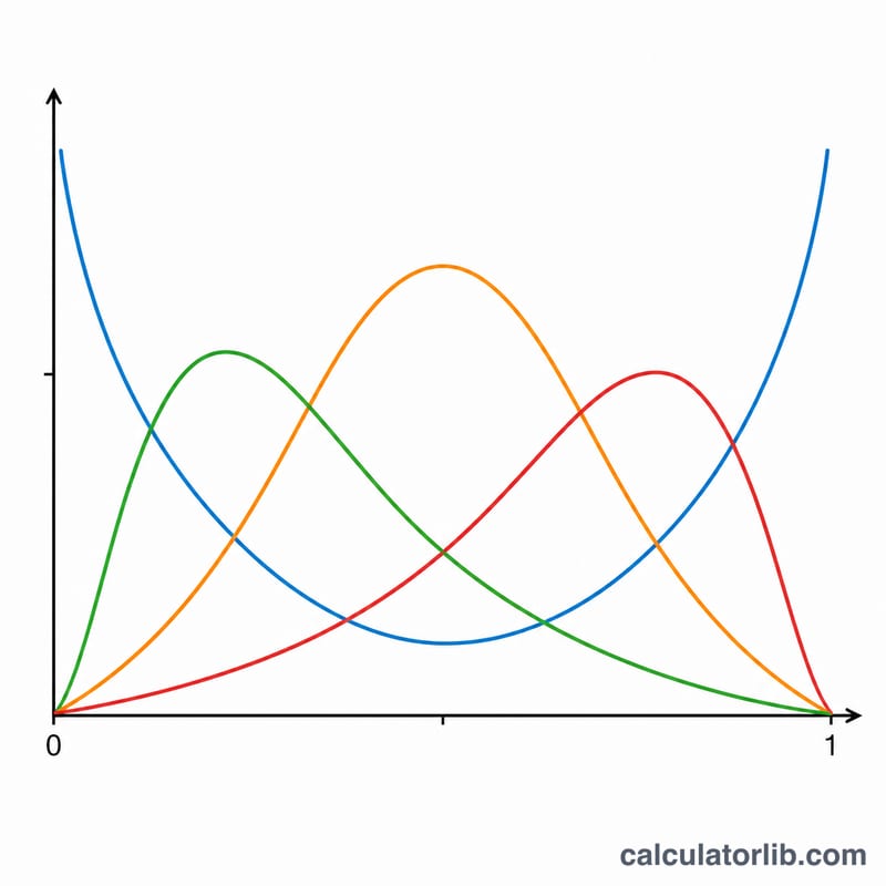
Enter your two shape parameters α and β (both must be greater than 0) and a value x between 0 and 1. The calculator returns the probability density f(x) at that point, along with the distribution's mean, variance, standard deviation and mode. Larger α pushes mass toward 1; larger β pushes mass toward 0; equal values make it symmetric around 0.5.
The Formula Explained
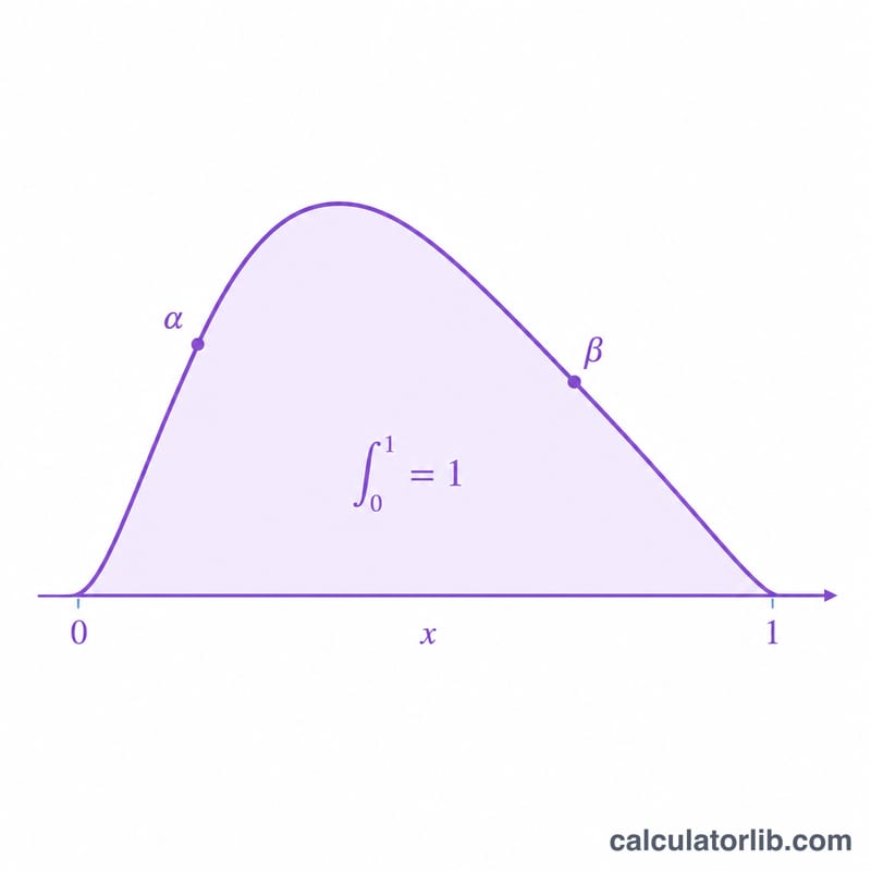
The mean is \(\mu = \frac{\alpha}{\alpha+\beta}\) and the variance is \(\sigma^2 = \frac{\alpha\,\beta}{\left(\alpha+\beta\right)^2\left(\alpha+\beta+1\right)}\). The probability density is $$f(\text{x};\,\alpha,\beta) = \frac{\text{x}^{\,\alpha-1}\left(1-\text{x}\right)^{\beta-1}}{B\!\left(\alpha,\beta\right)}$$ where \(B(\alpha, \beta) = \frac{\Gamma(\alpha)\Gamma(\beta)}{\Gamma(\alpha + \beta)}\) is the Beta function that normalizes the curve so its total area equals 1. The mode (peak) exists at \(\frac{\alpha - 1}{\alpha + \beta - 2}\) when both α and β exceed 1.
Worked Example
Take α = 2, β = 5, x = 0.5. The mean is \(2/7 \approx 0.2857\). The variance is $$\frac{2\cdot 5}{(7^2)(8)} = \frac{10}{392} \approx 0.02551$$ With \(B(2, 5) = 1/30\), the density is $$f(0.5) = 0.5^1 \cdot 0.5^4 \cdot 30 = 0.5^5 \cdot 30 = 0.03125 \cdot 30 = 0.9375$$
How Shape Parameters Change the Distribution
The Beta distribution lives on the interval \([0,1]\) and its entire shape is controlled by the two positive shape parameters \(\alpha\) and \(\beta\). The mean is always \(\mu = \dfrac{\alpha}{\alpha+\beta}\), the variance is \(\sigma^2 = \dfrac{\alpha\beta}{(\alpha+\beta)^2(\alpha+\beta+1)}\), and the mode (when \(\alpha,\beta>1\)) is \(\dfrac{\alpha-1}{\alpha+\beta-2}\). The table below shows several classic parameter pairs.
| (α, β) | Shape | Mean = α/(α+β) | Mode | Variance |
|---|---|---|---|---|
| (1, 1) | Uniform (flat) on [0,1] | 0.5 | none (flat) | 0.0833 |
| (0.5, 0.5) | U-shaped (mass at both ends, arcsine) | 0.5 | 0 and 1 (antimodes) | 0.1250 |
| (2, 2) | Symmetric bell, peaked at center | 0.5 | 0.5 | 0.0500 |
| (5, 5) | Tighter symmetric bell | 0.5 | 0.5 | 0.0227 |
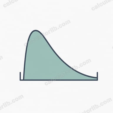
| (2, 5) | Right-skewed (mass toward 0) | 0.2857 | 0.2 | 0.0255 |
| (5, 2) | Left-skewed (mass toward 1) | 0.7143 | 0.8 | 0.0255 |
Two patterns stand out. First, swapping \(\alpha\) and \(\beta\) mirrors the distribution about \(x=0.5\), so (2,5) and (5,2) have the same shape and variance but opposite skew. Second, increasing both parameters while keeping their ratio fixed (e.g. (2,2) \(\to\) (5,5)) keeps the mean at 0.5 but shrinks the variance, concentrating the curve more tightly around the mean.
Interpreting Your Beta Result
Because the Beta distribution is supported on \([0,1]\), it is the natural model for an unknown proportion, probability or rate. Each summary statistic answers a different question:
- Mean \(\mu=\alpha/(\alpha+\beta)\) is the expected proportion — your best single-number estimate of the underlying probability.
- Mode \((\alpha-1)/(\alpha+\beta-2)\) is the most likely value, i.e. the location of the peak of the density. It exists as an interior peak only when \(\alpha>1\) and \(\beta>1\); otherwise the mass piles up at an endpoint.
- Variance and standard deviation measure spread, or how much uncertainty remains about the proportion. A small SD means you are confident the true value lies near the mean.
The quantity \(\alpha+\beta\) acts like a sample size or concentration: the larger it is, the smaller the variance and the more sharply the density concentrates around the mean. Two distributions can share the same mean yet have very different certainty — Beta(2,2) and Beta(50,50) are both centered at 0.5, but the latter is far narrower.
In Bayesian inference the Beta is the conjugate prior for a binomial (Bernoulli) likelihood. If you start with a prior Beta(\(\alpha_0,\beta_0\)) and then observe \(s\) successes and \(f\) failures, the posterior is simply Beta(\(\alpha_0+s,\ \beta_0+f\)). With a uniform Beta(1,1) prior, \(\alpha\) effectively counts successes \(+1\) and \(\beta\) counts failures \(+1\); the posterior mean \((s+1)/(s+f+2)\) is the classic Laplace rule of succession.
Finally, remember that \(f(x)\) is a probability density, not a probability. Its value can exceed 1 (for example near the peak of a tightly concentrated Beta), and only the area under the curve between two points — never the height at a single point — gives an actual probability. The total area over \([0,1]\) always equals 1.
Definitions & Glossary
- α (alpha)
- The first shape parameter, \(\alpha>0\). Loosely it represents the weight of "successes"; larger \(\alpha\) pushes mass toward 1.
- β (beta)
- The second shape parameter, \(\beta>0\). Loosely it represents the weight of "failures"; larger \(\beta\) pushes mass toward 0.
- PDF f(x)
- The probability density function, \(f(x;\alpha,\beta)=\dfrac{x^{\alpha-1}(1-x)^{\beta-1}}{B(\alpha,\beta)}\) for \(0\le x\le 1\). It describes relative likelihood; probabilities are areas under it.
- Beta function B(α,β)
- The normalizing constant, \(B(\alpha,\beta)=\displaystyle\int_0^1 t^{\alpha-1}(1-t)^{\beta-1}\,dt=\dfrac{\Gamma(\alpha)\Gamma(\beta)}{\Gamma(\alpha+\beta)}\). Dividing by it makes the density integrate to 1.
- Gamma function Γ
- A continuous extension of the factorial, \(\Gamma(n)=(n-1)!\) for positive integers, defined generally by \(\Gamma(z)=\int_0^\infty t^{z-1}e^{-t}\,dt\). It links the Beta and Gamma functions above.
- Mean
- The expected value, \(\mu=\dfrac{\alpha}{\alpha+\beta}\) — the long-run average proportion.
- Variance
- A measure of spread, \(\sigma^2=\dfrac{\alpha\beta}{(\alpha+\beta)^2(\alpha+\beta+1)}\).
- Standard deviation
- The square root of the variance, \(\sigma=\sqrt{\sigma^2}\), expressed in the same units as \(x\).
- Mode
- The most likely value (peak of the density), \(\dfrac{\alpha-1}{\alpha+\beta-2}\) when \(\alpha>1\) and \(\beta>1\).
- Conjugate prior
- A prior distribution that, combined with a given likelihood, yields a posterior in the same family. Beta is the conjugate prior for the binomial/Bernoulli likelihood.
- Support [0,1]
- The range of values the random variable can take. The Beta distribution is defined only on the closed interval \([0,1]\), making it ideal for proportions and probabilities.
FAQ
Can α or β be less than 1? Yes — values below 1 produce a U- or J-shaped curve with density spiking toward the endpoints. Density at the boundaries may then be unbounded.
When is the Beta distribution uniform? When α = β = 1 the PDF is flat and equals 1 everywhere on [0, 1] — identical to the uniform distribution.
Why must x stay between 0 and 1? The Beta distribution has zero density outside [0, 1], so values beyond this range are undefined for the PDF.