Bayes' Theorem Calculator

Total probability P(B)	0.0882
Formula	P(A\|B) = P(B\|A)·P(A) / P(B)

What Is Bayes' Theorem?

Bayes' theorem describes how to update the probability of a hypothesis A in light of new evidence B. It converts a prior belief into a posterior belief by weighing how likely the evidence is under the hypothesis against how likely it is overall. It is foundational to statistics, machine learning, medical diagnostics, spam filtering, and rational decision-making under uncertainty.

How to Use This Calculator

Enter three probabilities, each between 0 and 1:

P(A) — the prior probability that the hypothesis is true (e.g. the base rate of a disease).
P(B|A) — the likelihood: the probability of seeing the evidence when A is true (e.g. test sensitivity).
P(B|¬A) — the false-positive rate: the probability of the evidence when A is false.

The calculator derives the total probability of the evidence $P(B)$ automatically using the law of total probability, then returns the posterior $P(A \mid B)$.

The Formula Explained

The core equation is

$$P(A \mid B) = \frac{P(B \mid A) \cdot P(A)}{P(B)}$$

Because $P(B)$ is rarely known directly, we expand it as

$$P(B) = P(B \mid A) \cdot P(A) + P(B \mid \neg A) \cdot (1 - P(A))$$

This combines the true-positive and false-positive contributions to find how often the evidence appears at all.

Tree diagram branching from a root into two hypothesis branches, each splitting into positive and negative test outcomes — A probability tree showing how the prior splits into likelihood and false-positive branches.

Worked Example

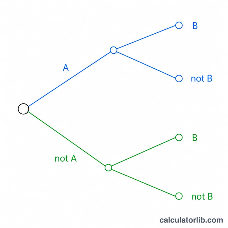
Suppose a disease affects 1% of people, so $P(A) = 0.01$. A test correctly flags sick people 90% of the time, $P(B \mid A) = 0.9$, but also has an 8% false-positive rate, $P(B \mid \neg A) = 0.08$. Then

$$P(B) = 0.9 \times 0.01 + 0.08 \times 0.99 = 0.009 + 0.0792 = 0.0882$$

The posterior is

$$P(A \mid B) = \frac{0.009}{0.0882} \approx 0.102$$

or about 10.2%. Despite a "positive" test, the patient is probably healthy — a classic illustration of base-rate neglect.

Two overlapping rectangles representing populations, with the overlap region highlighted to show the posterior — Visualizing the posterior as the highlighted overlap relative to all positive results.

How the Posterior Changes Across Scenarios

Bayes' theorem combines a prior probability $P(A)$, a true-positive rate (likelihood) $P(B \mid A)$, and a false-positive rate $P(B \mid \neg A)$ into an updated posterior $P(A \mid B)$. The single most surprising feature of the result is its sensitivity to the base rate $P(A)$: when a condition is rare, even a highly accurate test produces a low posterior. The table below holds the test characteristics fixed in places and varies the inputs to make that dependence visible.

Scenario	Prior P(A)	Likelihood P(B\|A)	False-positive P(B\|¬A)	Posterior P(A\|B)
Rare condition, accurate test	0.01	0.99	0.05	0.1667
Rare condition, lower false-positive rate	0.01	0.99	0.01	0.5
Moderate base rate, accurate test	0.10	0.99	0.05	0.6875
Common condition, accurate test	0.50	0.99	0.05	0.9519
Rare condition, high false-positive rate	0.01	0.90	0.20	0.0435

Reading down the first two rows shows that cutting the false-positive rate from 0.05 to 0.01 raises the posterior from about 17% to 50% even though the base rate and sensitivity are unchanged. Reading rows one, three and four shows that as the prior rises from 1% to 50%, the same test pushes the posterior from 17% all the way to about 95%. The last row demonstrates the opposite extreme: a rare condition combined with a high false-positive rate keeps the posterior under 5% despite a 90% true-positive rate.

Interpreting Your Posterior Probability

The posterior $P(A \mid B)$ is the probability that hypothesis $A$ is true after you have observed evidence $B$. It answers the practical question "given this positive result, how likely is the condition actually present?" — which is usually what a decision-maker wants to know.

It is important not to confuse the posterior with the likelihood $P(B \mid A)$. The likelihood (often called sensitivity or the true-positive rate in a testing context) is the probability of seeing the evidence assuming $A$ is true. These two conditional probabilities point in opposite directions, and they are only equal in special cases. A test can have a 99% true-positive rate yet yield a posterior far below 99% — the difference is driven by the base rate and the false-positive rate.

The base rate $P(A)$ is the engine behind this gap. When $A$ is rare, the pool of true cases is small, so even a modest false-positive rate applied to the large $\neg A$ population can generate more false positives than true positives. Ignoring the base rate and reading a positive result as near-certain is the well-known base-rate fallacy.

Finally, Bayesian updating is iterative. Once you compute a posterior, it can serve as the prior for the next piece of independent evidence. Observing a second positive test, for instance, means you feed the first posterior back in as $P(A)$ and update again. Repeated independent evidence steadily refines the estimate, which is why Bayesian reasoning underlies sequential testing, spam filtering, and many machine-learning models.

Key Terms and Variables

Prior — $P(A)$: The probability assigned to hypothesis $A$ before observing the evidence. In testing contexts this is the prevalence or base rate of the condition.
Likelihood — $P(B \mid A)$: The probability of observing evidence $B$ when $A$ is true. For a diagnostic test this is the sensitivity or true-positive rate.
False-positive rate — $P(B \mid \neg A)$: The probability of observing evidence $B$ when $A$ is false. It equals $1 - \text{specificity}$ for a diagnostic test.
Evidence / marginal likelihood — $P(B)$: The total probability of observing the evidence under all hypotheses, computed by the law of total probability as $P(B) = P(B \mid A)\,P(A) + P(B \mid \neg A)\,\bigl(1 - P(A)\bigr)$. It is the denominator that normalizes the posterior.
Posterior — $P(A \mid B)$: The updated probability of $A$ after accounting for evidence $B$. It is the output of Bayes' theorem.
Base rate: Another name for the prior $P(A)$ — the underlying frequency of the hypothesis in the population, independent of any specific test result.
Bayes' theorem: The rule relating these quantities: $P(A \mid B) = \dfrac{P(B \mid A)\,P(A)}{P(B)}$. The notation $P(X \mid Y)$ reads "the probability of $X$ given $Y$," and $\neg A$ denotes "not $A$," the complement of the hypothesis.

FAQ

Why is the posterior so low in the example? Because the disease is rare, far more healthy people generate false positives than sick people generate true positives.

What if I already know $P(B)$? You can adjust $P(B \mid \neg A)$ so that the computed total matches, but this tool always derives $P(B)$ from the law of total probability for consistency.

Do the inputs need to sum to 1? No. Each is an independent probability between 0 and 1; only $P(A)$ and $(1 - P(A))$ are complementary.