Máy Tính Định Lý Bayes

Tổng xác suất P(B)	0,0882
Công thức	P(A\|B) = P(B\|A)·P(A) / P(B)

Định lý Bayes là gì?

Định lý Bayes mô tả cách cập nhật xác suất của một giả thuyết A khi xuất hiện bằng chứng mới B. Nó biến niềm tin tiên nghiệm (prior) thành niềm tin hậu nghiệm (posterior) bằng cách cân nhắc xem bằng chứng có khả năng xảy ra đến đâu nếu giả thuyết đúng, so với khả năng xảy ra của bằng chứng nói chung. Đây là nền tảng của thống kê, học máy (machine learning), chẩn đoán y khoa, lọc thư rác và việc ra quyết định hợp lý trong điều kiện bất định.

Cách sử dụng công cụ này

Nhập ba giá trị xác suất, mỗi giá trị nằm trong khoảng từ 0 đến 1:

P(A) — xác suất tiên nghiệm rằng giả thuyết đúng (ví dụ: tỷ lệ mắc bệnh trong dân số).
P(B|A) — độ khả dĩ: xác suất quan sát thấy bằng chứng khi A đúng (ví dụ: độ nhạy của xét nghiệm).
P(B|¬A) — tỷ lệ dương tính giả: xác suất xuất hiện bằng chứng khi A sai.

Công cụ sẽ tự động suy ra tổng xác suất của bằng chứng $P(B)$ bằng công thức xác suất toàn phần, sau đó trả về xác suất hậu nghiệm $P(A|B)$.

Giải thích công thức

Phương trình cốt lõi là $$P(A \mid B) = \frac{\text{P(B|A)} \cdot \text{P(A)}}{\text{P(B|A)} \cdot \text{P(A)} + \text{P(B|¬A)} \cdot \left(1 - \text{P(A)}\right)}$$ Vì hiếm khi biết trực tiếp $P(B)$, ta khai triển nó thành $$P(B) = P(B|A) \cdot P(A) + P(B|¬A) \cdot (1 - P(A))$$ Cách này gộp cả phần đóng góp của dương tính thật và dương tính giả để xác định bằng chứng xuất hiện thường xuyên đến mức nào.

Quảng cáo

Sơ đồ cây phân nhánh từ gốc thành hai giả thuyết, mỗi nhánh lại chia thành kết quả xét nghiệm dương tính và âm tính — Cây xác suất cho thấy xác suất tiên nghiệm tách thành các nhánh khả năng và dương tính giả.

Ví dụ minh họa

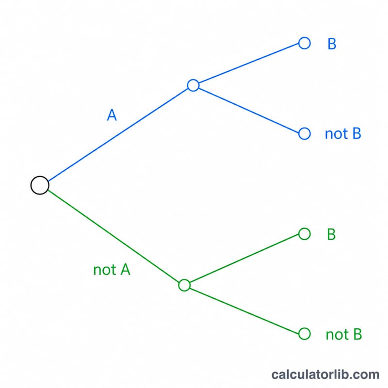
Giả sử một căn bệnh ảnh hưởng đến 1% dân số, tức $P(A) = 0{,}01$. Xét nghiệm phát hiện đúng người bệnh 90% số lần, $P(B|A) = 0{,}9$, nhưng cũng có tỷ lệ dương tính giả 8%, $P(B|¬A) = 0{,}08$. Khi đó $$P(B) = 0{,}9 \times 0{,}01 + 0{,}08 \times 0{,}99 = 0{,}009 + 0{,}0792 = 0{,}0882$$ Xác suất hậu nghiệm là $$P(A|B) = 0{,}009 / 0{,}0882 \approx 0{,}102$$ tức khoảng 10,2%. Dù kết quả xét nghiệm "dương tính", bệnh nhân nhiều khả năng vẫn khỏe mạnh — một minh họa kinh điển cho hiện tượng bỏ qua tỷ lệ nền (base-rate neglect).

Hai hình chữ nhật chồng lên nhau biểu thị các quần thể, với vùng giao nhau được tô sáng để thể hiện xác suất hậu nghiệm — Trực quan hóa xác suất hậu nghiệm dưới dạng vùng giao nhau được tô sáng so với tất cả kết quả dương tính.

Cách Hậu Xác Suất Thay Đổi Across Scenarios

Bayes' theorem combines a prior probability $P(A)$, a true-positive rate (likelihood) $P(B \mid A)$, and a false-positive rate $P(B \mid \neg A)$ into an updated posterior $P(A \mid B)$. The single most surprising feature of the result is its sensitivity to the base rate $P(A)$: when a condition is rare, even a highly accurate test produces a low posterior. The table below holds the test characteristics fixed in places and varies the inputs to make that dependence visible.

Scenario	Prior P(A)	Likelihood P(B\|A)	False-positive P(B\|¬A)	Posterior P(A\|B)
Rare condition, accurate test	0.01	0.99	0.05	0.1667
Rare condition, lower false-positive rate	0.01	0.99	0.01	0.5
Moderate base rate, accurate test	0.10	0.99	0.05	0.6875
Common condition, accurate test	0.50	0.99	0.05	0.9519
Rare condition, high false-positive rate	0.01	0.90	0.20	0.0435

Reading down the first two rows shows that cutting the false-positive rate from 0.05 to 0.01 raises the posterior from about 17% to 50% even though the base rate and sensitivity are unchanged. Reading rows one, three and four shows that as the prior rises from 1% to 50%, the same test pushes the posterior from 17% all the way to about 95%. The last row demonstrates the opposite extreme: a rare condition combined with a high false-positive rate keeps the posterior under 5% despite a 90% true-positive rate.

Giải Thích Xác Suất Hậu Của Bạn

The posterior $P(A \mid B)$ is the probability that hypothesis $A$ is true after you have observed evidence $B$. It answers the practical question "given this positive result, how likely is the condition actually present?" — which is usually what a decision-maker wants to know.

It is important not to confuse the posterior with the likelihood $P(B \mid A)$. The likelihood (often called sensitivity or the true-positive rate in a testing context) is the probability of seeing the evidence assuming $A$ is true. These two conditional probabilities point in opposite directions, and they are only equal in special cases. A test can have a 99% true-positive rate yet yield a posterior far below 99% — the difference is driven by the base rate and the false-positive rate.

The base rate $P(A)$ is the engine behind this gap. When $A$ is rare, the pool of true cases is small, so even a modest false-positive rate applied to the large $\neg A$ population can generate more false positives than true positives. Ignoring the base rate and reading a positive result as near-certain is the well-known base-rate fallacy.

Finally, Bayesian updating is iterative. Once you compute a posterior, it can serve as the prior for the next piece of independent evidence. Observing a second positive test, for instance, means you feed the first posterior back in as $P(A)$ and update again. Repeated independent evidence steadily refines the estimate, which is why Bayesian reasoning underlies sequential testing, spam filtering, and many machine-learning models.

Quảng cáo

Các Thuật Ngữ và Biến Chính

Prior — $P(A)$: The probability assigned to hypothesis $A$ before observing the evidence. In testing contexts this is the prevalence or base rate of the condition.
Likelihood — $P(B \mid A)$: The probability of observing evidence $B$ when $A$ is true. For a diagnostic test this is the sensitivity or true-positive rate.
False-positive rate — $P(B \mid \neg A)$: The probability of observing evidence $B$ when $A$ is false. It equals $1 - \text{specificity}$ for a diagnostic test.
Evidence / marginal likelihood — $P(B)$: The total probability of observing the evidence under all hypotheses, computed by the law of total probability as $P(B) = P(B \mid A)\,P(A) + P(B \mid \neg A)\,\bigl(1 - P(A)\bigr)$. It is the denominator that normalizes the posterior.
Posterior — $P(A \mid B)$: The updated probability of $A$ after accounting for evidence $B$. It is the output of Bayes' theorem.
Base rate: Another name for the prior $P(A)$ — the underlying frequency of the hypothesis in the population, independent of any specific test result.
Bayes' theorem: The rule relating these quantities: $P(A \mid B) = \dfrac{P(B \mid A)\,P(A)}{P(B)}$. The notation $P(X \mid Y)$ reads "the probability of $X$ given $Y$," and $\neg A$ denotes "not $A$," the complement of the hypothesis.

Câu hỏi thường gặp

Vì sao xác suất hậu nghiệm trong ví dụ lại thấp đến vậy? Vì căn bệnh hiếm gặp, nên số người khỏe mạnh cho ra kết quả dương tính giả nhiều hơn nhiều so với số người bệnh cho ra kết quả dương tính thật.

Nếu tôi đã biết sẵn $P(B)$ thì sao? Bạn có thể điều chỉnh $P(B|¬A)$ sao cho tổng tính ra khớp với giá trị đó, nhưng để đảm bảo nhất quán, công cụ này luôn suy ra $P(B)$ từ công thức xác suất toàn phần.

Các giá trị nhập vào có cần cộng lại bằng 1 không? Không. Mỗi giá trị là một xác suất độc lập nằm trong khoảng từ 0 đến 1; chỉ có $P(A)$ và $(1 - P(A))$ là bù trừ cho nhau.