What this calculator does
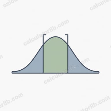
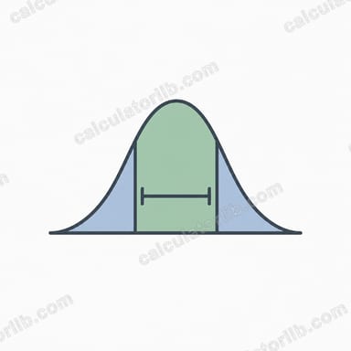
This calculator finds the k factor and the tolerance limits \(\bar{Y} \pm k s\) for data assumed to come from a normal distribution. A tolerance interval is a range expected, with a stated confidence, to contain at least a stated proportion of the whole population, not just of the sample. It suits engineers, quality analysts and researchers who need to describe where most individual values will fall.

How to use it
Choose the interval type: two-sided, or one-sided (a lower and an upper limit, each independent). Enter the sample mean, the sample standard deviation (n-1 divisor, zero or more), and the sample size N (a whole number, at least 2). Enter the coverage proportion p and the confidence level as proportions strictly between 0 and 1, for example 0.90 and 0.99. Mean and standard deviation must be valid numbers; entries that cannot be read as numbers should be corrected before calculating.
Formula
Two-sided factor (Howe approximation):
$$k_2 = z_{(1+p)/2}\sqrt{\frac{\nu\,(1+1/N)}{\chi^2_{1-\gamma,\nu}}}$$One-sided factor (Natrella):
$$k_1=\frac{z_p+\sqrt{z_p^2-ab}}{a},\quad a=1-\frac{z_\gamma^2}{2(N-1)},\quad b=z_p^2-\frac{z_\gamma^2}{N}$$Limits:
$$\bar{Y}-ks \quad\text{and}\quad \bar{Y}+ks$$Here \(p\) = coverage, \(\gamma\) = confidence, \(N\) = sample size, \(\nu = N-1\) = degrees of freedom, \(z_q\) = standard normal quantile at cumulative probability q, \(\chi^2_{1-\gamma,\nu}\) = chi-square quantile at cumulative probability \(1-\gamma\), \(\bar{Y}\) = sample mean and \(s\) = sample standard deviation.
Conventions and assumptions
- The two-sided k uses Howe's 1969 approximation as given in the NIST/SEMATECH handbook. The chi-square term is the lower quantile at probability 1 minus confidence, which matches the handbook example (column 0.01, 42 degrees of freedom, 23.650).
- The handbook calls the confidence level alpha; here it is called confidence and entered as a proportion.
- Guenther's correction is not applied; the plain Howe factor is returned.
- The one-sided k uses the Natrella formulas, which need only normal quantiles. The non-central t method is not offered.
- Degrees of freedom are N-1, since one sample estimates both mean and standard deviation.
- In one-sided mode the lower and upper limits are separate one-sided bounds, not a two-sided pair. Coverage must be at least 0.5.
- Quantiles come from double-precision inverse distribution functions, not rounded tables. The k factor and limits are shown to 4 decimals.
Worked example
Two-sided, \(N=43\), \(p=0.90\), \(\gamma=0.99\), mean 100, \(s=5\). Then \(\nu=42\) and
$$k_2 = 2.2173$$The limits are:
$$100 - 2.2173\times 5 = 88.9134$$$$100 + 2.2173\times 5 = 111.0866$$With 99% confidence, at least 90% of the population lies between 88.9134 and 111.0866. The degrees of freedom are 42.
Reading the result and limitations
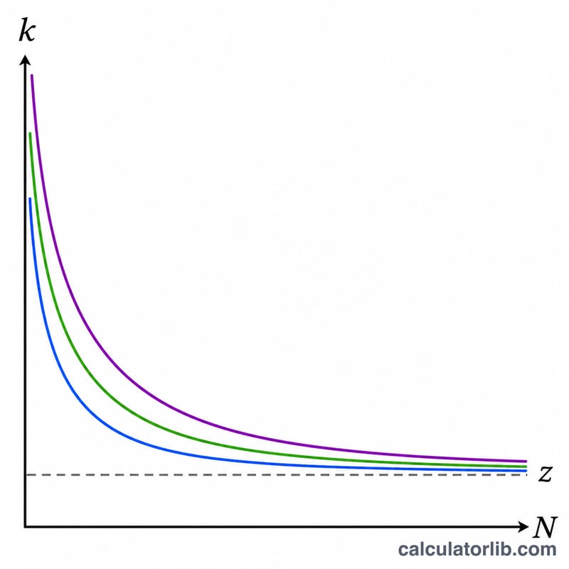
A larger k gives a wider interval. The k factor shrinks toward the normal quantile as N grows, and rises with higher coverage or confidence. The results assume normality and random sampling; heavy tails or outliers invalidate them. For small samples (N of 10 or fewer) the one-sided Natrella approximation is noticeably less accurate than the non-central t method; the source gives 5.2808 versus 4.4111 for N = 6. For very small N with high p or confidence, no real k may exist and the sample size must be increased. A standard deviation of zero gives limits equal to the mean.
FAQ
How does a tolerance interval differ from a confidence interval?
A confidence interval estimates a parameter such as the mean. A tolerance interval bounds a stated proportion of individual values in the population.
What do coverage and confidence mean?
Coverage is the minimum proportion of the population the interval should contain. Confidence is the long-run probability that intervals built this way achieve that coverage.
Why is the one-sided mode giving an error?
The approximation can have no real solution for very small samples with high coverage or confidence. Increase N or lower the levels.
Can I use it for non-normal data?
Not reliably. Check normality first or transform the data.
Why do my results differ slightly from printed tables?
Tables are rounded and may use exact factors; this tool computes the approximations directly in double precision.
Sources
- 7.2.6.3. Tolerance intervals for a normal distribution, NIST/SEMATECH e-Handbook of Statistical Methods