What is the Associated Legendre Polynomial Table Calculator?
This tool computes a table of values of the associated Legendre function \(P_n^m(x)\) (degree \(n\), order \(m\)) over a chosen range of \(x\) and draws the corresponding curve. It is pure mathematics and applies identically everywhere, with no units or country-specific assumptions. The associated Legendre polynomials appear throughout physics and applied mathematics: in spherical harmonics, the solution of Laplace's equation in spherical coordinates, multipole expansions, and quantum mechanics of angular momentum.
How to use it
Enter the integer degree \(n\) (0, 1, 2, ...) and the integer order \(m\) with \(-n \le m \le n\). Choose the start value of \(x\) (between -1 and 1), the step increment, and the number of rows. The defaults \(n = 2\), \(m = 1\), start = -1, step = 0.02, 101 rows sweep \(x\) from -1 to +1 inclusive. Select Type A (Wolfram convention) or Type B (Maple convention); for real \(x\) in \((-1, 1)\) they agree in magnitude and differ only by a sign/phase of the prefactor.
The formula explained
For integer \(n\) and \(0 \le m \le n\) we use $$P_n^m(x) = (-1)^m(1-x^2)^{m/2}\,\frac{d^m}{dx^m}P_n(x),$$ evaluated with the numerically stable recurrence $$P_m^m = (-1)^m(2m-1)!!(1-x^2)^{m/2},$$ $$P_{m+1}^m = x(2m+1)P_m^m,$$ then $$(l-m)P_l^m = (2l-1)x\,P_{l-1}^m - (l+m-1)P_{l-2}^m.$$ For negative \(m\), $$P_n^{-m} = (-1)^m\frac{(n-m)!}{(n+m)!}P_n^m.$$ This closed recurrence avoids the Gamma-function blow-up of the literal \({}_2F_1\) form for positive integer \(m\).
Worked example
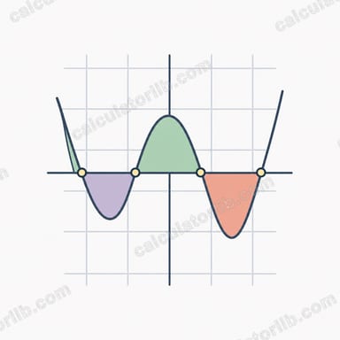
With \(n = 2\), \(m = 1\) the function is $$P_2^1(x) = -3x\sqrt{1-x^2}.$$ At \(x = 0\) the value is 0; at \(x = 0.5\) it is $$-3(0.5)(0.866025) = -1.299038;$$ at \(x = -0.5\) it is \(+1.299038\). The curve starts at 0 (\(x = -1\)), rises to about \(+1.1547\) near \(x = -0.577\), crosses zero at \(x = 0\), dips to about \(-1.1547\) near \(x = +0.577\), and returns to 0 at \(x = +1\).
Closed-Form Associated Legendre Functions P_n^m(x)
The associated Legendre functions \(P_n^m(x)\) for integer degree \(n\) and order \(0\le m\le n\) follow from \(P_n^m(x)=(-1)^m(1-x^2)^{m/2}\dfrac{d^m}{dx^m}P_n(x)\). The factor \((-1)^m\) is the Condon–Shortley phase included in the Type A convention (matching Wolfram); the Type B convention (Maple) omits it, so its odd-\(m\) entries differ only in sign. The table below lists the explicit forms under Type A.
| \(n\) | \(m\) | \(P_n^m(x)\) (Type A, with sign) |
|---|---|---|
| 0 | 0 | \(1\) |
| 1 | 0 | \(x\) |
| 1 | 1 | \(-\sqrt{1-x^2}\) |
| 2 | 0 | \(\tfrac{1}{2}(3x^2-1)\) |
| 2 | 1 | \(-3x\sqrt{1-x^2}\) |
| 2 | 2 | \(3(1-x^2)\) |
| 3 | 0 | \(\tfrac{1}{2}(5x^3-3x)\) |
| 3 | 1 | \(-\tfrac{3}{2}(5x^2-1)\sqrt{1-x^2}\) |
| 3 | 2 | \(15x(1-x^2)\) |
| 3 | 3 | \(-15(1-x^2)^{3/2}\) |
As a worked check, at \(x=0.5\) the entry \(P_2^1\) gives \(-3(0.5)\sqrt{1-0.25}=-1.5\sqrt{0.75}=\) -1.299038. The \(m=0\) column reproduces the ordinary Legendre polynomials \(P_n(x)\), e.g. \(P_3^0(x)=\tfrac12(5x^3-3x)\), which can be tabulated with the Legendre polynomial table calculator.
Key Terms and Variables
- Degree \(n\)
-
A non-negative integer (
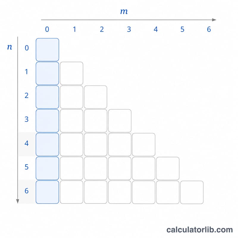
degreeN) setting the order of the underlying Legendre polynomial \(P_n(x)\), which is a polynomial of degree \(n\). - Order \(m\)
-
An integer (
orderM) controlling how many derivatives are taken. For real-valued results on \((-1,1)\) one normally uses \(0\le m\le n\); when \(m>n\) the function is identically zero because the \(m\)-th derivative of a degree-\(n\) polynomial vanishes. - Argument \(x\)
-
The evaluation point (
initialXplus \(i\cdot\)stepX). The functions are real for \(-1\le x\le 1\); in physics \(x=\cos\theta\). - Type A (Wolfram / Condon–Shortley)
-
Includes the phase factor \((-1)^m\). This is the convention used by Wolfram's
LegendrePand standard quantum-mechanics texts. - Type B (Maple)
- Omits the \((-1)^m\) phase, so \(P_n^m\) (Type B) \(=(-1)^m\,P_n^m\) (Type A). Magnitudes are identical; only the sign of odd-\(m\) entries differs.
- Double factorial \((2m-1)!!\)
- The product of odd integers \((2m-1)(2m-3)\cdots 3\cdot 1\), with \((-1)!!=1\). It appears in the leading coefficient \(P_m^m(x)=(-1)^m(2m-1)!!\,(1-x^2)^{m/2}\); e.g. \(P_3^3\) uses \(5!!=15\). See the double-factorial calculator for these values.
- Negative-order relation
- For \(m>0\), \(P_n^{-m}(x)=(-1)^m\dfrac{(n-m)!}{(n+m)!}\,P_n^{m}(x)\), connecting positive and negative orders through factorials.
Interpreting the Table and Graph
Several structural properties let you sanity-check the tabulated values and the plotted curve:
- Parity. \(P_n^m(-x)=(-1)^{n+m}P_n^m(x)\). When \(n+m\) is even the graph is symmetric about \(x=0\); when \(n+m\) is odd it is antisymmetric (and therefore passes through the origin).
- Zeros in the interior. On the open interval \((-1,1)\), \(P_n^m(x)\) has exactly \(n-m\) simple zeros. For example \(P_3^1\) has two interior zeros, while \(P_n^n\) has none.
- Endpoint behavior. Because of the factor \((1-x^2)^{m/2}\), every function with \(m>0\) vanishes at \(x=\pm 1\). For \(m=0\) the values are \(P_n(1)=1\) and \(P_n(-1)=(-1)^n\).
- Magnitude near the edges. For higher \(m\) the \((1-x^2)^{m/2}\) factor suppresses the curve sharply as \(x\to\pm1\), so the largest excursions occur toward the middle of the range.
These functions are the \(\theta\)-dependent part of the spherical harmonics \(Y_n^m(\theta,\phi)\): writing \(x=\cos\theta\), one has \(Y_n^m\propto P_n^m(\cos\theta)\,e^{im\phi}\). The interior zeros become the nodal circles of latitude, and the \(m>0\) endpoint vanishing corresponds to the harmonics tending to zero at the poles. The same \(P_n^m\) values therefore feed directly into a spherical-harmonics evaluation at a chosen \(\theta\) and \(\phi\).
FAQ
Why must \(n\) and \(m\) be integers? The terminating polynomial form requires a non-negative integer \(n\); the recurrence and the \((n\pm m)!\) factors require integer \(m\) with \(-n \le m \le n\).
What is the sample value shown? The hero box reports \(x\) and \(P_n^m(x)\) at the middle row of the table (the median index), a quick spot-check of the curve.
What does \(m = 0\) give? \(P_n^0(x)\) is the ordinary Legendre polynomial \(P_n(x)\).