
What is the Laguerre Polynomial Table Calculator?
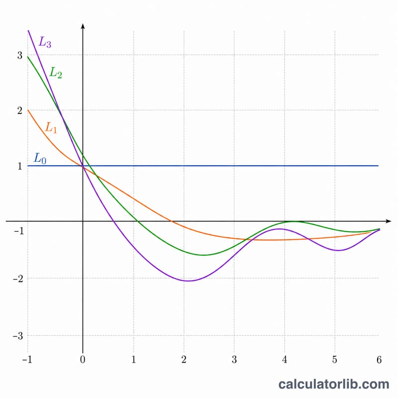
This tool tabulates and plots the Laguerre polynomial \(L_n(x)\) over a sequence of x values. The Laguerre polynomials are the orthogonal-polynomial solutions of the differential equation \(x\cdot y'' + (1 - x)\cdot y' + n\cdot y = 0\), and they appear throughout quantum mechanics (the radial part of the hydrogen atom), numerical integration (Gauss-Laguerre quadrature), and signal processing. This calculator uses the standard normalization with \(L_n(0) = 1\).
How to use it
Enter four numbers: the order n (a non-negative integer), the initial value of x, the increment (step) between successive x values, and the number of rows. The calculator generates \(x = \text{startX},\ \text{startX} + \text{stepX},\ \text{startX} + 2\cdot\text{stepX},\ \ldots\) and evaluates \(L_n(x)\) at each, returning a two-column table and a line graph.
The formula explained
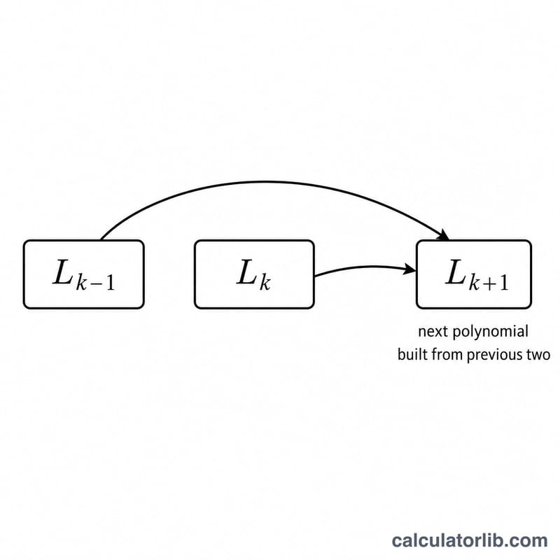
Rather than expanding the polynomial, the calculator uses the numerically stable three-term recurrence: \(L_0(x) = 1\), \(L_1(x) = 1 - x\), and for \(k \ge 1\), $$L_{k+1}(x) = \frac{(2k + 1 - x)\cdot L_k(x) - k\cdot L_{k-1}(x)}{k + 1}.$$ This requires only \(O(n)\) work per point. The first few polynomials are \(L_2(x) = 1 - 2x + \frac{x^2}{2}\) and \(L_3(x) = 1 - 3x + 1.5x^2 - \frac{x^3}{6}\).
Worked example
For \(n = 3\) and \(x = -1\): $$L_3(-1) = 1 + 3 + 1.5 + 0.16667 = 5.66667.$$ Checking with the recurrence: \(L_0 = 1\), \(L_1 = 2\), \(L_2 = 3.5\), $$L_3 = \frac{6\cdot 3.5 - 2\cdot 2}{3} = \frac{17}{3} = 5.66667.$$ At \(x = 0\), \(L_3(0) = 1\); at \(x = 1\), \(L_3(1) = -0.66667\).
FAQ
What normalization is used? The standard form with \(L_n(0) = 1\), not the unnormalized \(n!\cdot L_n(x)\) seen in some references.
What if n = 0? \(L_0(x) = 1\) everywhere, a flat horizontal line. For \(n = 1\) you get the straight line \(1 - x\).
How large can n be? The recurrence is stable for moderate \(n\). For very large \(n\) or large \(|x|\) the values grow rapidly and floating-point overflow may eventually occur.