What is the Chebyshev polynomial of the second kind?
The Chebyshev polynomials of the second kind, written \(U_n(x)\), are a family of orthogonal polynomials that appear throughout approximation theory, numerical analysis, and physics. This is a pure-mathematics tool: it works identically everywhere and is not tied to any country or jurisdiction. This calculator builds a table of values of \(U_n(x)\) over a chosen range of x and lets you visualize the resulting curve.
How to use it
Enter the order n (a non-negative integer), the initial value of x, the increment (spacing between successive x values), and the repeat count (how many sample points to generate). The table is produced for \(x = \text{startX},\ \text{startX} + \text{stepX},\ \text{startX} + 2 \times \text{stepX}\), and so on. With the defaults (n = 3, start = -1, step = 0.02, 101 points), x runs from -1 to 1.00.
The formula explained
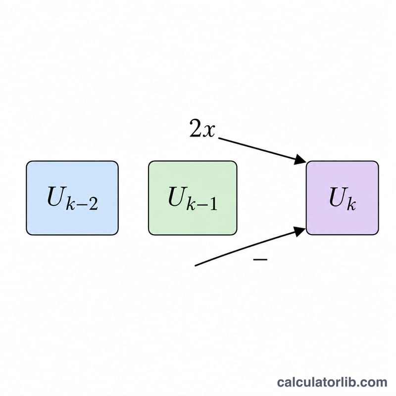
Rather than the trigonometric form $$U_n(\cos\theta) = \frac{\sin((n+1)\theta)}{\sin\theta}$$ (which divides by zero at \(x = \pm 1\)), this tool uses the stable three-term recurrence: \(U_0(x) = 1\), \(U_1(x) = 2x\), and $$U_k(x) = 2x \cdot U_{k-1}(x) - U_{k-2}(x).$$ The recurrence is exact for every real x and lets values grow naturally for \(|x| > 1\). The polynomials satisfy the ODE $$(1 - x^2)y'' - 3xy' + n(n+2)y = 0.$$
Worked example
For n = 3, the closed form is \(U_3(x) = 8x^3 - 4x\). At \(x = 0.5\): \(U_0 = 1\), \(U_1 = 1\), \(U_2 = 2(0.5)(1) - 1 = 0\), \(U_3 = 2(0.5)(0) - 1 = -1\). The closed form gives $$8(0.125) - 4(0.5) = 1 - 2 = -1.$$ At the endpoints, \(U_n(1) = n+1\) so \(U_3(1) = 4\), and \(U_n(-1) = (-1)^n(n+1)\) so \(U_3(-1) = -4\).
FAQ
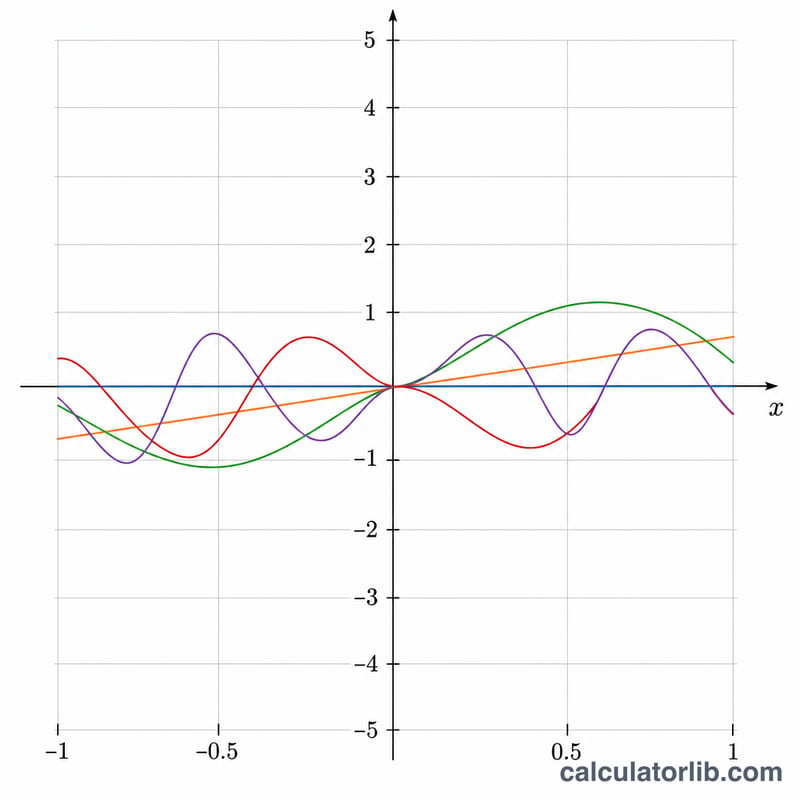
What are the first few polynomials? \(U_0 = 1\), \(U_1 = 2x\), \(U_2 = 4x^2 - 1\), \(U_3 = 8x^3 - 4x\), \(U_4 = 16x^4 - 12x^2 + 1\).
Can x be outside [-1, 1]? Yes. The polynomial is defined for all real x; the recurrence handles \(|x| > 1\) cleanly, though values grow rapidly.
What if n is not a whole number? The order is floored to a non-negative integer; negative values are clamped to 0.