What is the Gegenbauer (Ultraspherical) Polynomial?
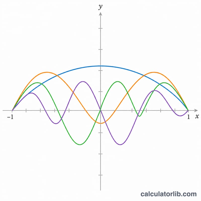
The Gegenbauer polynomials, also called ultraspherical polynomials, are a family of orthogonal polynomials \(C_{n}^{\lambda}(x)\) that generalize both the Legendre and Chebyshev polynomials. They are orthogonal on the interval [-1, 1] with weight \((1 - x^{2})^{\lambda-1/2}\). This calculator evaluates \(C_{n}^{\lambda}(x)\) across many x values at once, building a table of (x, value) pairs and a line graph that you can use to study the polynomial's shape, roots, and oscillation.
How to Use It
Enter the degree n (a non-negative integer), the parameter λ (real; standard orthogonality needs λ > -1/2), the initial value of x, the increment (spacing between successive x values), and the number of repetitions (how many rows to generate). The calculator iterates $$x_i = \text{initialX} + i\cdot\text{stepX}$$ for \(i = 0 \dots \text{count}-1\) and evaluates the polynomial at each point. The defaults (n=3, λ=2, x from -1, step 0.02, 101 rows) sweep the full orthogonality window from -1 to +1.
The Formula Explained
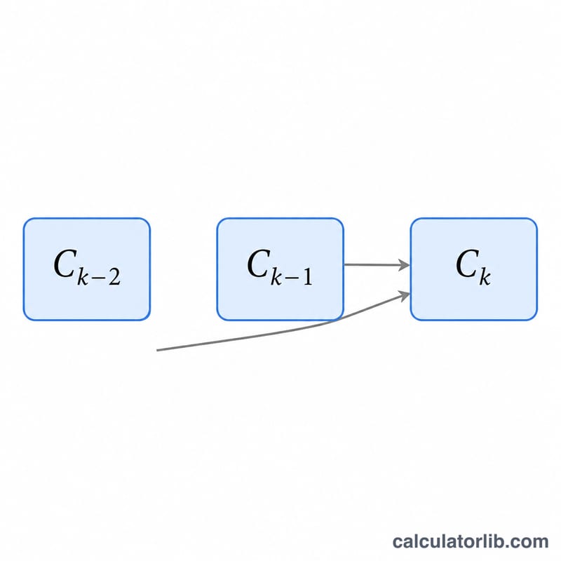
Rather than the gamma/hypergeometric form, the calculator uses the numerically stable three-term recurrence: \(C_{0}^{\lambda}(x) = 1\), \(C_{1}^{\lambda}(x) = 2\lambda x\), and for \(k = 2 \dots n\), $$C_{k}^{\lambda}(x) = \frac{2x(k+\lambda-1)\,C_{k-1}^{\lambda}(x) - (k+2\lambda-2)\,C_{k-2}^{\lambda}(x)}{k}.$$ Special cases: \(\lambda = 1/2\) gives Legendre polynomials \(P_{n}\), and \(\lambda = 1\) gives Chebyshev polynomials of the second kind \(U_{n}\).
Worked Example
With n=3 and λ=2 the recurrence yields \(C_{3}^{2}(x) = 32x^{3} - 12x\). At \(x = -1\), that is $$32(-1) - 12(-1) = -32 + 12 = -20,$$ which is the first table row. At \(x = 0\) the value is 0, at \(x = 0.5\) it is \(32(0.125) - 6 = -2\), and at \(x = 1\) it is \(32 - 12 = 20\).
FAQ
Is the polynomial defined outside [-1, 1]? Yes. The polynomial is defined for all real x; the interval [-1, 1] is just where the orthogonality (and the default graph window) lives. Outside it, values grow rapidly for higher n.
What happens at λ = 0? This is the degenerate ultraspherical case: the recurrence collapses, so the calculator returns \(C_{0} = 1\) and \(C_{n} = 0\) for \(n \ge 1\). The meaningful limit relates to Chebyshev of the first kind via \(\lim_{\lambda\to 0} C_{n}^{\lambda}(x)/\lambda = (2/n)\,T_{n}(x)\).
How many rows can I generate? Pick any count \(\ge 1\); the tool caps very large requests for responsiveness. The increment may be zero (all rows share the same x) but is normally positive.