What this calculator does
This tool tabulates the associated (generalized) Laguerre polynomial \(L_{n}^{(\alpha)}(x)\) over a sequence of x values. You provide the degree n, the parameter α, a starting x, a step size, and how many rows to generate. The calculator returns the value of the polynomial at each x. It is pure mathematics and applies universally — no region- or country-specific assumptions.
How to use it
Enter n (a non-negative integer), α (any real number; the standard orthogonality case uses \(\alpha > -1\)), the initial value of x, the increment, and the number of rows. The x values are generated as $$x_i = \text{startX} + i \times \text{stepX}$$ for \(i = 0, 1, \dots, \text{count}-1\), and each value \(L_{n}^{(\alpha)}(x_i)\) is computed and listed.
The formula explained
The closed form is a finite sum, $$L_{n}^{(\alpha)}(x) = \sum_{k=0}^{n} (-1)^k \binom{n+\alpha}{n-k} \frac{x^k}{k!},$$ where \(\binom{n+\alpha}{n-k}\) is the generalized binomial coefficient. For numerical stability the calculator instead uses the three-term recurrence: $$L_0 = 1,\quad L_1 = 1 + \alpha - x,\quad (k+1)L_{k+1} = (2k+1+\alpha-x)L_{k} - (k+\alpha)L_{k-1}.$$ This avoids large factorials and cancellation for moderate-to-large n.
Worked example
With the defaults \(n = 3\), \(\alpha = 1\) the explicit polynomial is $$L_{3}^{(1)}(x) = 4 - 6x + 2x^2 - \tfrac{1}{6}x^3.$$ At \(x = 0\) the value is \(4\). At \(x = 0.1\) it is $$4 - 0.6 + 0.02 - 0.0001667 \approx 3.419833.$$ At \(x = 1\) it equals $$4 - 6 + 2 - 0.166667 = -0.166667.$$
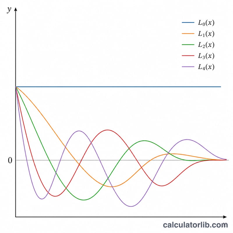
First Associated Laguerre Polynomials
The associated (generalized) Laguerre polynomials \(L_n^{(\alpha)}(x)\) are polynomials of degree \(n\) in \(x\) whose coefficients depend on the parameter \(\alpha\). The closed form is
$$L_n^{(\alpha)}(x)=\sum_{k=0}^{n}(-1)^k\binom{n+\alpha}{n-k}\frac{x^k}{k!}.$$The first five, written in general \(\alpha\) form, are:
| \(n\) | \(L_n^{(\alpha)}(x)\) |
|---|---|
| 0 | \(1\) |
| 1 | \(-x+(\alpha+1)\) |
| 2 | \(\dfrac{x^2}{2}-(\alpha+2)x+\dfrac{(\alpha+1)(\alpha+2)}{2}\) |
| 3 | \(-\dfrac{x^3}{6}+\dfrac{(\alpha+3)x^2}{2}-\dfrac{(\alpha+2)(\alpha+3)x}{2}+\dfrac{(\alpha+1)(\alpha+2)(\alpha+3)}{6}\) |
| 4 | \(\dfrac{x^4}{24}-\dfrac{(\alpha+4)x^3}{6}+\dfrac{(\alpha+3)(\alpha+4)x^2}{4}-\dfrac{(\alpha+2)(\alpha+3)(\alpha+4)x}{6}+\dfrac{(\alpha+1)(\alpha+2)(\alpha+3)(\alpha+4)}{24}\) |
Special case \(\alpha=0\). Setting \(\alpha=0\) recovers the ordinary Laguerre polynomials \(L_n(x)=L_n^{(0)}(x)\):
| \(n\) | \(L_n(x)\) |
|---|---|
| 0 | \(1\) |
| 1 | \(1-x\) |
| 2 | \(1-2x+\tfrac12 x^2\) |
| 3 | \(1-3x+\tfrac32 x^2-\tfrac16 x^3\) |
| 4 | \(1-4x+3x^2-\tfrac23 x^3+\tfrac{1}{24}x^4\) |
The leading coefficient is always \(\dfrac{(-1)^n}{n!}\), independent of \(\alpha\).
Key Terms & Variables
- Degree \(n\)
- A non-negative integer giving the polynomial degree; \(L_n^{(\alpha)}(x)\) has exactly \(n\) roots. In the calculator this is the field degree.
- Parameter \(\alpha\)
- A real number (commonly \(\alpha>-1\)) that shifts the binomial coefficients and the orthogonality weight. The field alpha. With \(\alpha=0\) the polynomials reduce to the ordinary Laguerre polynomials.
- Argument \(x\)
- The point at which the polynomial is evaluated. The table sweeps \(x_i=\text{startX}+i\cdot\text{stepX}\). The natural domain for orthogonality is \((0,\infty)\).
- Generalized binomial coefficient
- For real upper index, \(\binom{n+\alpha}{n-k}=\dfrac{\Gamma(n+\alpha+1)}{\Gamma(k+\alpha+1)\,(n-k)!}\), which extends \(\binom{m}{j}=m!/(j!(m-j)!)\) to non-integer \(\alpha\) via the Gamma function.
- Three-term recurrence
- The stable way to generate the polynomials: \((k+1)L_{k+1}^{(\alpha)}=(2k+1+\alpha-x)L_k^{(\alpha)}-(k+\alpha)L_{k-1}^{(\alpha)}\), starting from \(L_0^{(\alpha)}=1\) and \(L_1^{(\alpha)}=1+\alpha-x\).
- Orthogonality on \((0,\infty)\)
- The polynomials are mutually orthogonal: \(\displaystyle\int_0^\infty L_n^{(\alpha)}(x)L_m^{(\alpha)}(x)\,w(x)\,dx=\frac{\Gamma(n+\alpha+1)}{n!}\delta_{nm}\).
- Weight function \(w(x)=x^{\alpha}e^{-x}\)
- The factor against which orthogonality holds; for \(\alpha=0\) it is the simple exponential weight \(e^{-x}\). Convergence of the integral requires \(\alpha>-1\).
Interpreting the Table
Reading a computed table of \(L_n^{(\alpha)}(x)\) becomes easier with these facts:
- Number of real roots. For \(\alpha>-1\), \(L_n^{(\alpha)}(x)\) has exactly \(n\) simple real zeros, all lying in the open interval \((0,\infty)\). If your table column crosses zero \(n\) times, you have located all of them.
- Sign changes. Because all zeros are simple, the polynomial changes sign at each one. Between two consecutive zeros the values keep a constant sign, so a sign flip between adjacent rows brackets a root — useful as a starting interval for a bisection or Newton root finder.
- Value at the origin. Every associated Laguerre polynomial satisfies \(L_n^{(\alpha)}(0)=\binom{n+\alpha}{n}=\dfrac{\Gamma(n+\alpha+1)}{n!\,\Gamma(\alpha+1)}\). For example, with \(n=4,\ \alpha=0\) the first row at \(x=0\) is 1, and with \(n=4,\ \alpha=2\) it is \(\binom{6}{4}=\) 15.
- Quantum mechanics. The radial part of the hydrogen-atom wavefunction is built from \(L_{n-\ell-1}^{(2\ell+1)}\!\left(2r/(na_0)\right)\); the polynomial's nodes correspond to the radial nodes of the orbital.
- Gauss–Laguerre quadrature. The zeros listed in the table are exactly the abscissae used to approximate \(\int_0^\infty f(x)\,x^{\alpha}e^{-x}\,dx\), with weights derived from the same polynomials.
This is general mathematical reference information; verify any value you rely on in a critical application.
FAQ
What if n = 0? \(L_{0}^{(\alpha)}(x) = 1\) for every x and every α.
Can α be negative or non-integer? Yes — both the sum and the recurrence work for any real α. The classical orthogonality on \((0, \infty)\) requires \(\alpha > -1\).
Can the step be zero or negative? Yes. A negative step walks x downward; a zero step repeats the same x and produces a degenerate (constant-x) table.