What this calculator does
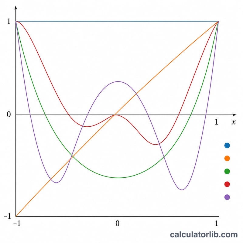
This tool builds a table of values for the Legendre polynomial \(P_n(x)\) for a chosen degree \(n\), evaluated over a sequence of x values, and draws the corresponding curve. You pick the degree, a starting x, a step increment, and how many rows you want; the calculator returns each pair \((x, P_n(x))\) plus a line plot. Legendre polynomials are a classic family of orthogonal polynomials on the interval [-1, 1] and appear throughout physics and applied mathematics — in solutions of Laplace's equation, multipole expansions, spherical harmonics, and Gaussian quadrature.
How to use it
Enter n (degree) as a non-negative integer (0, 1, 2, …). Set the initial value of x (often -1), the increment (step) between successive x values (e.g. 0.02), and the number of repetitions (rows) you want generated. The i-th row uses \(x = \text{startX} + i \times \text{step}\). Although the polynomials are most meaningful on [-1, 1], the formula works for any real x — note that outside that interval the magnitude grows quickly.
The formula explained
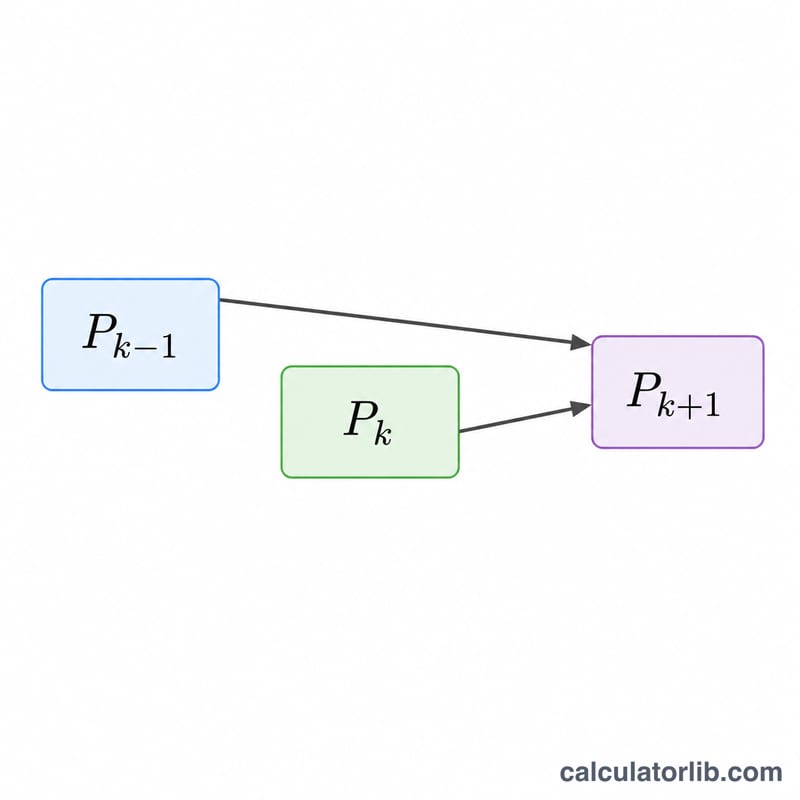
Rather than expanding closed forms, the calculator uses Bonnet's recursion for numerical stability: start with \(P_0(x) = 1\) and \(P_1(x) = x\), then iterate
$$P_{k+1}(x) = \frac{(2k+1)\cdot x\cdot P_k(x) - k\cdot P_{k-1}(x)}{k+1}.$$The first closed forms are \(P_2 = \frac{3x^2 - 1}{2}\), \(P_3 = \frac{5x^3 - 3x}{2}\), and \(P_4 = \frac{35x^4 - 30x^2 + 3}{8}\).
Worked example
For \(n = 3\) at \(x = 0.5\): \(P_0 = 1\), \(P_1 = 0.5\). Then
$$P_2 = \frac{3\cdot 0.5\cdot 0.5 - 1}{2} = -0.125,$$$$P_3 = \frac{5\cdot 0.5\cdot(-0.125) - 2\cdot 0.5}{3} = \frac{-1.3125}{3} = -0.4375.$$The closed form \(\frac{5x^3 - 3x}{2}\) gives the same result, confirming the recursion.
FAQ
What does n = 0 give? A constant value of 1 for every x, so the graph is a flat horizontal line. What are the endpoint values? Every Legendre polynomial satisfies \(P_n(1) = 1\) and \(P_n(-1) = (-1)^n\). Why use the recursion instead of explicit formulas? The three-term recurrence is fast and numerically stable for arbitrary degree, avoiding the cancellation errors of high-order explicit polynomials.