What is the Bessel Y Function Table Calculator?
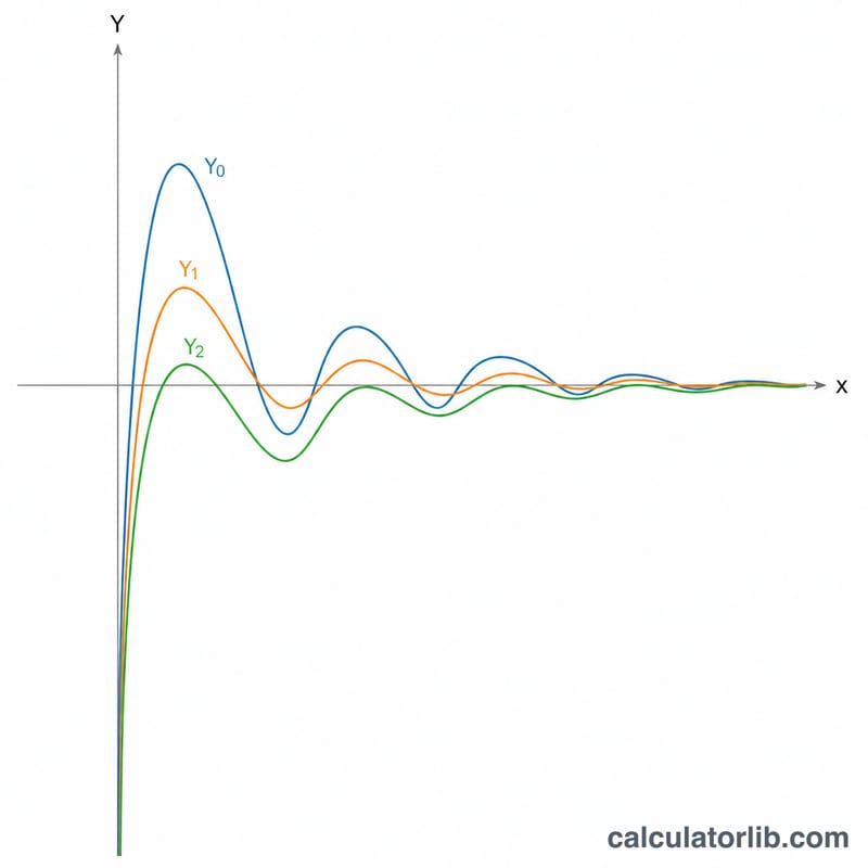
This tool tabulates the Bessel function of the second kind, also called the Weber or Neumann function, written \(Y_v(x)\). It is the second linearly independent solution of Bessel's differential equation. For a fixed real order v, the calculator evaluates \(Y_v(x)\) at a sequence of x values defined by a starting value, an increment, and a number of points, producing a full numeric table.
How to use it
Enter the order v (which may be non-integer or negative), the initial value of x, the increment (step) between points, and the number of iterations (rows). The calculator builds \(x_i = \text{startX} + i \cdot \text{stepX}\) for \(i = 0\) to \(\text{pointCount}-1\) and lists \(Y_v(x)\) for each. Note that \(Y_v(x)\) diverges to negative infinity at x = 0 and is real only for x > 0, so any x ≤ 0 row is marked undefined.
The formula
For non-integer order: $$Y_{\nu}(x) = \frac{J_{\nu}(x)\cos(\nu\pi) - J_{-\nu}(x)}{\sin(\nu\pi)}$$ For integer order n, the limit gives a closed form with a logarithmic term involving \(J_n(x)\cdot\ln(x/2)\), a finite power-series correction, and a digamma series. The first-kind function \(J_v(x)\) is summed from its power series, with the Gamma function evaluated by a Lanczos approximation.
Worked example
With v = 0, startX = 0, stepX = 0.2, pointCount = 51, the rows run x = 0.0 to 10.0. \(Y_0(0)\) is undefined (−∞), \(Y_0(0.2) \approx -1.0811\), \(Y_0(1.0) \approx 0.0883\), \(Y_0(2.0) \approx 0.5104\), and \(Y_0(10.0) \approx 0.0557\). The headline "first finite value" reports −1.0811.
Definitions & Glossary
- Order \(\nu\)
-
The parameter (the
orderfield) that indexes the family of Bessel functions. It may be any real number. Integer orders (0, 1, 2, …) are most common in physical problems with cylindrical symmetry; half-integer orders give spherical Bessel functions. - Bessel function of the second kind \(Y_\nu(x)\)
- Also called the Weber or Neumann function (sometimes written \(N_\nu\)). It is a solution of Bessel's equation that is unbounded (singular) at the origin. Defined for non-integer \(\nu\) by \(Y_\nu(x) = \dfrac{J_\nu(x)\cos(\nu\pi) - J_{-\nu}(x)}{\sin(\nu\pi)}\), with the integer case obtained as a limit.
- \(J_\nu\) versus \(Y_\nu\)
- \(J_\nu(x)\) (first kind) is finite at \(x=0\); \(Y_\nu(x)\) (second kind) diverges to \(-\infty\) as \(x\to 0^+\). Together they form a complete pair of independent solutions of Bessel's equation.
- Bessel's differential equation
- The linear ODE \(x^2 y'' + x y' + (x^2 - \nu^2) y = 0\). Its general solution is \(y = c_1 J_\nu(x) + c_2 Y_\nu(x)\).
- Gamma function \(\Gamma(z)\)
- The continuous extension of the factorial, \(\Gamma(n+1) = n!\), appearing in the series coefficients of \(J_\nu\) and \(Y_\nu\).
- Digamma function \(\psi(z)\)
- The logarithmic derivative \(\psi(z) = \Gamma'(z)/\Gamma(z)\). It appears explicitly in the series for integer-order \(Y_n(x)\), which contains a logarithmic term \(\tfrac{2}{\pi}\ln(x/2)J_n(x)\) plus digamma-weighted coefficients.
- Lanczos approximation
- A highly accurate numerical method for evaluating the gamma function \(\Gamma(z)\) for complex or real argument, commonly used inside Bessel-function routines to compute series coefficients.
- Linearly independent solution
- A second solution not expressible as a constant multiple of the first. Because \(J_\nu\) alone cannot represent solutions that are singular at the origin, \(Y_\nu\) supplies the independent companion needed for the general solution.
FAQ
Why is the first row undefined? \(Y_v(x)\) has a singularity at x = 0, diverging to −∞, so it has no finite value there.
Can the order be negative? Yes. For negative integer order the symmetry \(Y_{-n}(x) = (-1)^n Y_n(x)\) applies; for negative non-integer order the general formula is used directly.
How accurate is it? The series are summed until terms fall below machine tolerance, giving roughly 6-7 significant digits for moderate x.