What is the Struve function?
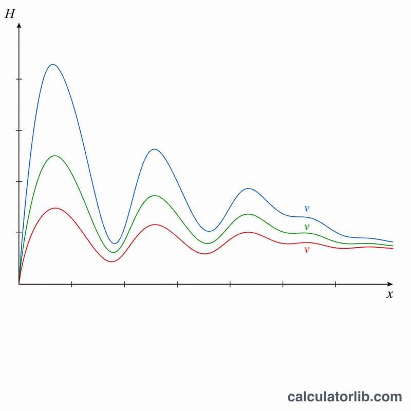
The Struve function \(\mathbf{H}_{v}(x)\) is a special function that arises as a particular solution of the inhomogeneous Bessel equation. It appears in problems of acoustics, fluid dynamics, optics and electromagnetics, often alongside the ordinary Bessel functions. This calculator tabulates \(\mathbf{H}_{v}(x)\) of any real order \(v\) across a chosen sequence of \(x\) values, so you can inspect its oscillating, slowly decaying behavior. It is pure mathematics and applies universally, with no regional or unit dependence.
How to use this calculator
Enter four values: the Order v (the order of the Struve function), the Initial value of x (the first argument), the Increment (the spacing between successive x values), and the Number of repetitions (how many rows to generate). The table then lists each argument \(x_{i} = \text{startX} + i \times \text{stepX}\) and the corresponding value \(\mathbf{H}_{v}(x_{i})\). With the defaults (\(v = 0\), start = -10, step = 0.2, count = 101) you get 101 points sweeping \(x\) from -10 to +10.
The formula explained
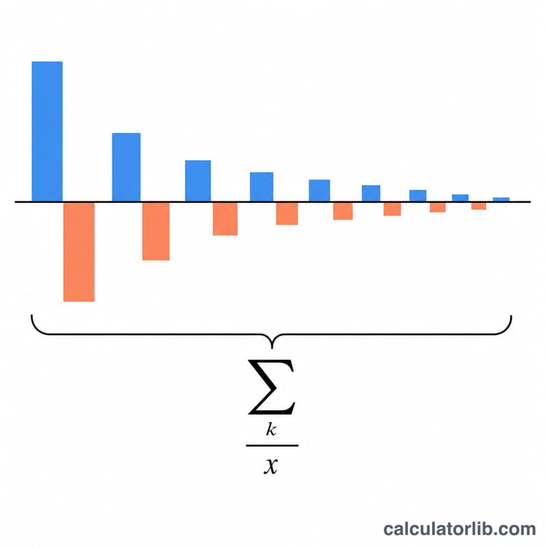
The value is evaluated directly from the power series shown above. Writing \(t = x/2\), the prefactor is \(t^{v+1}\) and each term is \((-1)^{k} t^{2k}\) divided by the product of two gamma functions, \(\Gamma(k + 3/2)\) and \(\Gamma(k + v + 3/2)\). The gamma function is computed with a numerically stable Lanczos approximation, using the reflection formula $$\Gamma(z) = \frac{\pi}{\sin(\pi z)\,\Gamma(1 - z)}$$ when its argument is non-positive. The alternating series converges quickly for moderate \(|x|\).
Worked example
Take \(v = 0\) and \(x = 2\), so \(t = 1\) and the prefactor is 1. Summing the series gives $$1.273240 - 0.565884 + 0.090542 - 0.007391 + 0.000365 - \ldots \approx 0.79066.$$ Hence \(\mathbf{H}_{0}(2) \approx 0.79066\), matching the standard reference value.
FAQ
What is \(\mathbf{H}_{v}(0)\)? For any order \(v > -1\) the prefactor \((x/2)^{v+1}\) vanishes at \(x = 0\), so \(\mathbf{H}_{v}(0) = 0\).
Can I use negative or non-integer orders? Yes. For negative \(x\) with non-integer \(v\) the function becomes complex, so those rows are reported as not-a-number; for \(v = 0\) or integer orders the whole table stays real.
How accurate is it? The direct series is highly accurate for the default range. For very large \(|x|\) (beyond about 30) many terms are needed and an asymptotic expansion would be preferable.


