
What is the Brillouin function?
The Brillouin function \(B_J(x)\) describes the magnetization of a paramagnet made of atoms with total angular momentum quantum number J. In statistical mechanics the dimensionless argument is \(x = \frac{g\cdot\mu_B\cdot J\cdot B}{k_B\cdot T}\), the ratio of magnetic to thermal energy. This calculator is a pure-math special-function evaluator: you supply x directly (no physical units), and it returns a table and a graph of \(B_J(x)\). When J becomes very large the function approaches the classical Langevin function \(L(x)\), which you can select by entering "inf".
How to use this calculator
Enter J as an integer, a half-integer fraction such as 1/2 or 3/2, or as a decimal like 0.5. Type "inf" for the Langevin limit. Then set the first x value (Initial value of x), the spacing between points (Increment), and how many rows to generate. The x values are produced as \(x_i = \text{startX} + i\cdot\text{stepX}\) for i = 0 to count−1. The tool prints every \((x, B_J(x))\) pair and draws the curve.
The formula explained
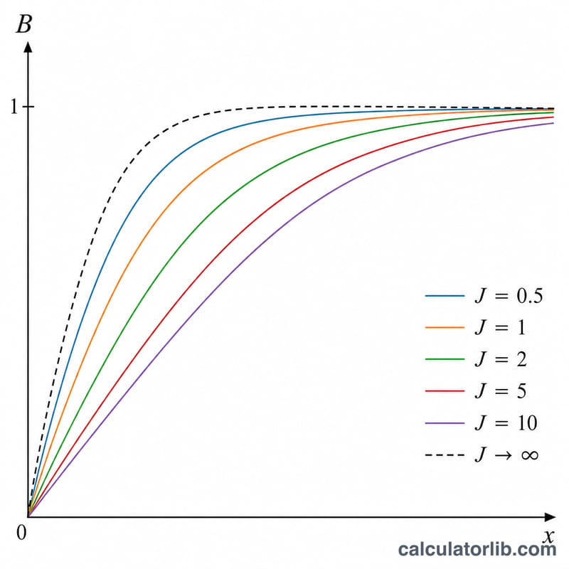
For finite J the function combines two hyperbolic cotangents: $$B_J(x) = \frac{2J+1}{2J}\coth\!\left(\frac{2J+1}{2J}\,x\right) - \frac{1}{2J}\coth\!\left(\frac{x}{2J}\right)$$ It is odd, so \(B_J(-x) = -B_J(x)\), passes through the origin (\(B_J(0)=0\)), and saturates to \(\pm 1\) as \(x \to \pm\infty\). Because coth has a singularity at zero, the calculator returns 0 for x at (or extremely close to) the origin, which is the correct analytic limit.
Worked example
Take J = 1/2 (so 2J = 1) at x = 1. Then \((2J+1)/2J = 2\) and \(1/2J = 1\), giving $$B_{1/2}(1) = 2\cdot\coth(2) - \coth(1) = 2(1.037314) - 1.313035 = 0.761594$$ As a check, for J = 1/2 the Brillouin function equals \(\tanh(x)\), and \(\tanh(1) = 0.761594\). For the Langevin case at x = 2: $$L(2) = \coth(2) - \frac{1}{2} = 1.037314 - 0.5 = 0.537314$$
Interpreting the Brillouin Function Result
The value returned by the calculator, \(B_J(x)\), is dimensionless and bounded between 0 and 1. Physically it equals the fractional magnetization of a paramagnet — the ratio of the actual magnetization to the saturation magnetization:
$$B_J(x) = \frac{M}{M_\text{sat}}, \qquad 0 \le B_J(x) \le 1.$$A result of 0 means no net alignment of magnetic moments (zero field or infinite temperature), while a result approaching 1 means every moment is fully aligned with the applied field (complete saturation).
The argument x: magnetic vs thermal energy
The input \(x\) is the ratio of the magnetic (Zeeman) energy of a moment to the available thermal energy:
$$x = \frac{g\,\mu_B\,J\,B}{k_B\,T}.$$When \(x\) is small the random thermal agitation \(k_B T\) dominates the aligning magnetic energy, so moments are nearly randomized; when \(x\) is large the magnetic energy wins and the moments lock into alignment.
Low-x (Curie) regime
For \(x \ll 1\) the Brillouin function is linear in \(x\):
$$B_J(x) \approx \frac{J+1}{3J}\,x.$$Substituting \(x = g\mu_B J B /(k_B T)\) gives a magnetization proportional to \(B/T\), which is exactly Curie's law: the susceptibility falls off as \(1/T\). This is the regime that applies to ordinary paramagnets in laboratory fields at room temperature, where \(B_J(x)\) is typically far below 1.
High-x saturation regime
For \(x \gg 1\) both hyperbolic cotangents tend to 1 and the function saturates:
$$B_J(x) \to 1.$$This corresponds to strong fields and/or very low temperatures, where essentially all magnetic moments point along the field and the magnetization can no longer increase. On the graph this appears as a plateau approaching the horizontal line \(B_J=1\). As \(J \to \infty\) the curve approaches the classical Langevin function \(L(x)=\coth x - 1/x\).
Key Terms and Variables
| Symbol / Term | Meaning |
|---|---|
| \(J\) | Total angular momentum quantum number of the magnetic ion (combines orbital and spin contributions). May be integer or half-integer (e.g. 1/2, 1, 3/2, 2). It sets the shape of the curve and the number of accessible \(m_J\) states, \(2J+1\). |
| \(x\) | Dimensionless argument of the function, \(x = g\mu_B J B/(k_B T)\) — the ratio of magnetic (Zeeman) energy to thermal energy. This is the horizontal axis of the table and graph. |
| \(g\) | Landé g-factor (spectroscopic splitting factor), a dimensionless number relating the magnetic moment to the angular momentum. For pure spin \(g \approx 2\); for combined orbital and spin angular momentum it is given by the Landé formula. |
| \(\mu_B\) | Bohr magneton, the natural unit of atomic magnetic moment, \(\mu_B = e\hbar/(2m_e) \approx 9.274\times10^{-24}\ \text{J/T}\). |
| \(k_B\) | Boltzmann constant, \(k_B \approx 1.381\times10^{-23}\ \text{J/K}\), converting temperature into thermal energy \(k_B T\). |
| \(B\) | Magnetic flux density (magnetic field), measured in tesla (T). Larger \(B\) increases \(x\) and drives the system toward saturation. |
| \(T\) | Absolute temperature in kelvin (K). Higher \(T\) increases thermal randomization, decreasing \(x\) and the magnetization. |
| \(\coth\) | Hyperbolic cotangent, \(\coth(u) = \cosh(u)/\sinh(u) = (e^{u}+e^{-u})/(e^{u}-e^{-u})\); it appears twice in the Brillouin function and tends to 1 for large \(u\). |
| Langevin function \(L(x)\) | The classical limit of the Brillouin function as \(J \to \infty\): \(L(x) = \coth x - 1/x\). It describes freely rotating classical magnetic dipoles (no quantization of orientation). |
FAQ
Why is \(B_J(0)\) shown as 0? Both coth terms diverge at x = 0 but their difference has the finite limit 0; the tool reports that limit.
What values of J are valid? Positive integers and half-integers (1/2, 1, 3/2, 2, ...). J = 0 is invalid because it divides by zero, and the calculator warns for non half-integer inputs.
How do I get the Langevin function? Enter "inf" (or "infinity") for J to use \(L(x) = \coth(x) - \frac{1}{x}\).


