Frobenius Norm Calculator
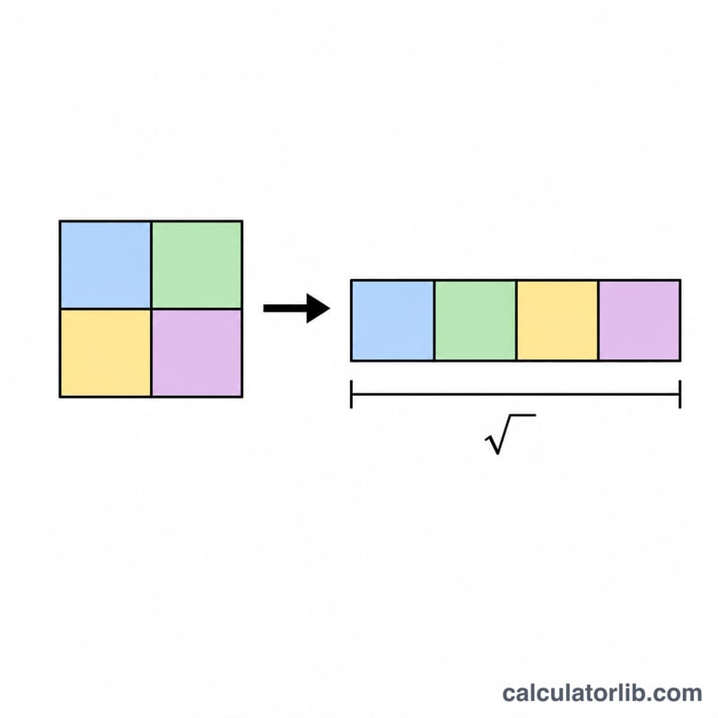
The Frobenius norm is a matrix norm that measures the magnitude of a matrix. It is calculated as the square root of the sum of the squared absolute values of all elements in the matrix. This calculator helps you compute the Frobenius norm of any matrix quickly and accurately.
What is the Frobenius Norm?
The Frobenius norm (also called the Euclidean norm) is a matrix norm defined as the square root of the sum of the squares of all the elements in a matrix. For a matrix A with elements \(a_{ij}\), the Frobenius norm is denoted as \(\lVert A \rVert_F\).
This norm provides a measure of the "size" of a matrix, similar to how the Euclidean norm measures the magnitude of a vector. It's widely used in linear algebra, matrix analysis, and numerical computations.
$$\lVert A \rVert_F = \sqrt{\sum_{i=1}^{m}\sum_{j=1}^{n} a_{ij}^{2}} \qquad A = \text{Matrix}$$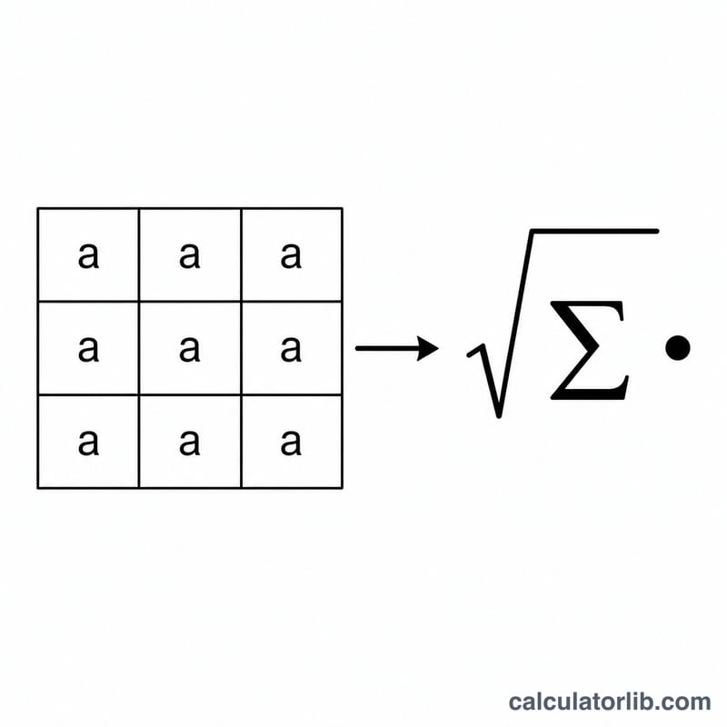
When to Use the Frobenius Norm
The Frobenius norm is particularly useful in various applications:
- Matrix Approximation: When measuring how close one matrix is to another in applications like low-rank approximations and compressed sensing.
- Numerical Analysis: For assessing the error or difference between matrices in iterative methods or numerical algorithms.
- Signal Processing: When analyzing the energy content of signals represented in matrix form.
Examples
Example 1: 2×2 Matrix
Calculate the Frobenius norm of the matrix A = [1, 2; 3, 4]
| Matrix | Calculation | Result |
|---|---|---|
| [1, 2; 3, 4] |
\(\sqrt{1^2 + 2^2 + 3^2 + 4^2} = \sqrt{1 + 4 + 9 + 16} = \sqrt{30}\) | 5.4772 |
Example 2: 3×3 Matrix
Calculate the Frobenius norm of the matrix B = [2, 0, 1; -1, 3, 5; 4, 2, 1]
| Matrix | Calculation | Result |
|---|---|---|
| [2, 0, 1; -1, 3, 5; 4, 2, 1] |
\(\sqrt{2^2 + 0^2 + 1^2 + (-1)^2 + 3^2 + 5^2 + 4^2 + 2^2 + 1^2} = \sqrt{4 + 0 + 1 + 1 + 9 + 25 + 16 + 4 + 1} = \sqrt{61}\) | 7.8102 |
Example 3: Non-square Matrix
Calculate the Frobenius norm of the 2×3 matrix C = [5, 2, 1; 3, 4, 0]
| Matrix | Calculation | Result |
|---|---|---|
| [5, 2, 1; 3, 4, 0] |
\(\sqrt{5^2 + 2^2 + 1^2 + 3^2 + 4^2 + 0^2} = \sqrt{25 + 4 + 1 + 9 + 16 + 0} = \sqrt{55}\) | 7.4162 |
Related Calculators
Explore these related matrix calculators for further analysis:
- Matrix Transpose Calculator - Compute the transpose of any matrix
- RREF Matrix Calculator - Find the Reduced Row Echelon Form of a matrix
- QR Factorization Calculator - Perform QR decomposition of matrices
- Cholesky Decomposition Calculator - Calculate the Cholesky decomposition of positive definite matrices
Related calculators
- Matrix Multiplication Calculator — multiply two matrices.
- Matrix Determinant Calculator — matrix determinant.
- Eigenvalue Calculator — eigenvalues of a 2x2 matrix.
- Dot Product Calculator — vector scalar product.
- Vector Magnitude Calculator — vector length.
How to Calculate the Frobenius Norm Step by Step
The Frobenius norm (also called the Hilbert–Schmidt or Euclidean matrix norm) is defined entrywise by the formula this calculator displays:
$$\lVert A \rVert_F = \sqrt{\sum_{i=1}^{m}\sum_{j=1}^{n} a_{ij}^{2}}$$- Write the matrix and note its dimensions. Record \(A\) with \(m\) rows and \(n\) columns, so it has \(m \times n\) entries in total. In the input box above, values within a row are separated by commas and rows are separated by
|. The limits \(i = 1 \ldots m\) and \(j = 1 \ldots n\) in the double sum are exactly these dimensions. - Square every entry. Replace each \(a_{ij}\) with \(a_{ij}^{2}\) — this is the term inside the double sum. Squaring removes signs, so \(-4\) and \(+4\) both contribute \(16\); the norm never depends on the sign pattern of the matrix. For a complex matrix, the correct term is the squared modulus \(|a_{ij}|^{2} = a_{ij}\,\overline{a_{ij}}\), which is real and non-negative (for example \(|3 + 4i|^2 = 9 + 16 = 25\)).
- Add all \(m \times n\) squared values. Work row by row: total the squares in row 1, then row 2, and so on, then add the row totals. That accumulation is the double sum \(\sum_{i}\sum_{j} a_{ij}^{2}\).
- Take the non-negative square root. Apply \(\sqrt{\;\cdot\;}\) to the sum. Because every term was a square, the sum is \(\ge 0\) and the principal (non-negative) root is always defined; \(\lVert A \rVert_F \ge 0\) by construction.
- Round to the desired precision. The square root is usually irrational, so report as many decimals as your application needs — and keep full precision in intermediate steps if the norm feeds into a further calculation.
Worked example
Take the \(2 \times 3\) matrix
$$A = \begin{bmatrix} 1 & -2 & 3 \\ 4 & 0 & -5 \end{bmatrix}$$Step 2 and 3, substituting every entry:
$$\sum_{i}\sum_{j} a_{ij}^{2} = 1^{2} + (-2)^{2} + 3^{2} + 4^{2} + 0^{2} + (-5)^{2} = 1 + 4 + 9 + 16 + 0 + 25 = 55$$Step 4 and 5:
$$\lVert A \rVert_F = \sqrt{55} \approx 7.416198$$So the Frobenius norm is 7.416198 (rounded to six decimals).
Two properties that simplify the work
- Order does not matter. Addition is commutative and associative, so the squared entries may be summed in any order — row by row, column by column, or all at once. The value of \(\lVert A \rVert_F\) is identical either way, which is why the norm is often described as "flattening" the matrix into a single list of numbers.
- Transposition changes nothing. Transposing swaps \(a_{ij}\) with \(a_{ji}\) but reuses exactly the same set of entries, so \(\lVert A \rVert_F = \lVert A^{\mathsf{T}} \rVert_F\). In the example above, the \(3 \times 2\) transpose also gives \(\sqrt{55}\).
A quick sanity check: the norm must be at least as large as the biggest absolute entry, since that entry's square is one of the terms in the sum. In the example, \(\sqrt{55} \approx 7.42 \ge 5\), as expected.
Key Terms and Notation
| Term | Symbol | Definition |
|---|---|---|
| Matrix | \(A\) | A rectangular array of numbers arranged in rows and columns. Its dimensions are written \(m \times n\), meaning \(m\) rows and \(n\) columns, for \(m \cdot n\) entries in total. |
| Element (entry) | \(a_{ij}\) | The single number located in row \(i\) and column \(j\) of \(A\). The first index always refers to the row. |
| Frobenius norm | \(\lVert A \rVert_F\) | The square root of the sum of the squares of all entries, \(\sqrt{\sum_i \sum_j a_{ij}^2}\). Also called the Hilbert–Schmidt norm or (in older texts) the Euclidean matrix norm. |
| Euclidean / vector 2-norm | \(\lVert x \rVert_2\) | For a vector \(x\), \(\sqrt{\sum_k x_k^2}\) — its ordinary length. If you flatten \(A\) into a single vector \(\mathrm{vec}(A)\) of length \(mn\), then \(\lVert A \rVert_F = \lVert \mathrm{vec}(A) \rVert_2\); the Frobenius norm is literally the vector 2-norm of the unrolled matrix. |
| Entrywise norm | — | A norm computed directly from the individual entries, treating the matrix as a list of numbers. The Frobenius norm is the entrywise 2-norm. |
| Induced (operator) norm | \(\lVert A \rVert_p\) | A norm defined by how much \(A\) can stretch a vector: \(\lVert A \rVert_p = \max_{x \ne 0} \lVert Ax \rVert_p / \lVert x \rVert_p\). Induced norms describe \(A\) as a map, not as a data array; the Frobenius norm is not an induced norm. |
| Spectral norm | \(\lVert A \rVert_2\) | The norm induced by the vector 2-norm, equal to the largest singular value \(\sigma_{\max}(A)\). Note the clash of notation: \(\lVert A \rVert_2\) for a matrix means the spectral norm, not the entrywise 2-norm. |
| Trace | \(\operatorname{trace}(A)\) | The sum of the diagonal entries of a square matrix, \(\sum_i a_{ii}\). It yields the identity \(\lVert A \rVert_F = \sqrt{\operatorname{trace}(A^{\mathsf{T}}A)}\) (use the conjugate transpose \(A^{*}\) for complex matrices), because the diagonal of \(A^{\mathsf{T}}A\) holds the squared column lengths. |
| Singular values | \(\sigma_i\) | The non-negative numbers on the diagonal of \(\Sigma\) in the singular value decomposition \(A = U\Sigma V^{\mathsf{T}}\). They satisfy \(\lVert A \rVert_F = \sqrt{\sum_i \sigma_i^2}\), so the Frobenius norm is the 2-norm of the singular-value vector. |
| Square vs non-square | \(m = n\) vs \(m \ne n\) | A square matrix has equally many rows and columns; a non-square (rectangular) one does not. The Frobenius norm is defined for both, unlike determinants or eigenvalues, which require \(m = n\). |
| Orthogonal / unitary invariance | \(Q^{\mathsf{T}}Q = I\) | An orthogonal matrix \(Q\) (real) or unitary matrix \(U\) (complex) preserves lengths and angles. The Frobenius norm is invariant under such multiplication: \(\lVert QAZ \rVert_F = \lVert A \rVert_F\) for orthogonal \(Q\) and \(Z\) of compatible size. |
| Rank | \(\operatorname{rank}(A)\) | The number of linearly independent rows (equivalently, columns) of \(A\), which equals the number of non-zero singular values. |
Interpreting Your Frobenius Norm Result
The number returned is a single non-negative magnitude summarizing the whole matrix. The following are established properties of that quantity.
Range and units
- \(\lVert A \rVert_F \ge 0\) always, and \(\lVert A \rVert_F = 0\) if and only if every entry is zero — that is, only for the zero matrix.
- It is not a probability, a percentage, or a score bounded by 1. There is no upper limit: the norm grows without bound as entries or dimensions grow.
- The result carries the units of the matrix entries, because squaring and then taking a square root returns to the original scale. If the entries are metres, the norm is in metres. Mixing entries of different physical units in one matrix makes the norm physically meaningless, even though the arithmetic still runs.
- The norm is at least as large as the largest absolute entry, \(\lVert A \rVert_F \ge \max_{i,j} |a_{ij}|\), and at most \(\sqrt{mn}\) times it.
How it responds to transformations
- Scaling: \(\lVert cA \rVert_F = |c| \cdot \lVert A \rVert_F\) for any scalar \(c\). Doubling every entry doubles the norm; negating the matrix leaves it unchanged.
- Transposition: \(\lVert A \rVert_F = \lVert A^{\mathsf{T}} \rVert_F\), since the same entries are summed.
- Orthogonal/unitary invariance: \(\lVert QA \rVert_F = \lVert AZ \rVert_F = \lVert A \rVert_F\) whenever \(Q\) and \(Z\) are orthogonal (or unitary). Rotations, reflections, and permutations of rows or columns therefore do not change the value.
- Triangle inequality and submultiplicativity: \(\lVert A + B \rVert_F \le \lVert A \rVert_F + \lVert B \rVert_F\), and \(\lVert AB \rVert_F \le \lVert A \rVert_F \cdot \lVert B \rVert_F\) for conformable \(A\) and \(B\).
Relation to the spectral norm
Because \(\lVert A \rVert_F = \sqrt{\sum_i \sigma_i^2}\) while \(\lVert A \rVert_2 = \sigma_{\max}\), the two norms are pinned together by
$$\lVert A \rVert_2 \;\le\; \lVert A \rVert_F \;\le\; \sqrt{\operatorname{rank}(A)} \cdot \lVert A \rVert_2$$The lower bound is attained when \(A\) has rank 1 (a single non-zero singular value), and the upper bound when all non-zero singular values are equal. For an \(n \times n\) identity matrix, for instance, \(\lVert I_n \rVert_2 = 1\) while \(\lVert I_n \rVert_F = \sqrt{n}\); with \(n = 4\) the Frobenius norm is 2.
As an approximation error
- \(\lVert A - B \rVert_F\) is the standard measure of how far one matrix is from another; it is the distance induced by the Frobenius inner product \(\langle A, B\rangle = \operatorname{trace}(A^{\mathsf{T}}B)\), and minimizing it is exactly least-squares fitting over all entries.
- The Eckart–Young–Mirsky theorem states that among all matrices \(B\) of rank at most \(k\), the truncated singular value decomposition \(A_k = \sum_{i=1}^{k} \sigma_i u_i v_i^{\mathsf{T}}\) minimizes \(\lVert A - B \rVert_F\), with the minimum value \(\lVert A - A_k \rVert_F = \sqrt{\sum_{i > k} \sigma_i^{2}}\). (The same truncation is also optimal in the spectral norm, where the error is \(\sigma_{k+1}\).)
Absolute versus relative size
A large value does not by itself indicate large entries — it may simply reflect a large matrix, since every one of the \(mn\) entries contributes. A matrix of 10,000 entries each equal to 0.1 has \(\lVert A \rVert_F = \sqrt{10000 \times 0.01} = 10\), despite every entry being small. For that reason the relative error
$$\frac{\lVert A - B \rVert_F}{\lVert A \rVert_F}$$is normally the meaningful quantity when comparing an approximation \(B\) to a reference \(A\); it is dimensionless and independent of the overall scale of \(A\). It is undefined when \(A\) is the zero matrix.