What is Gauss-Laguerre quadrature?
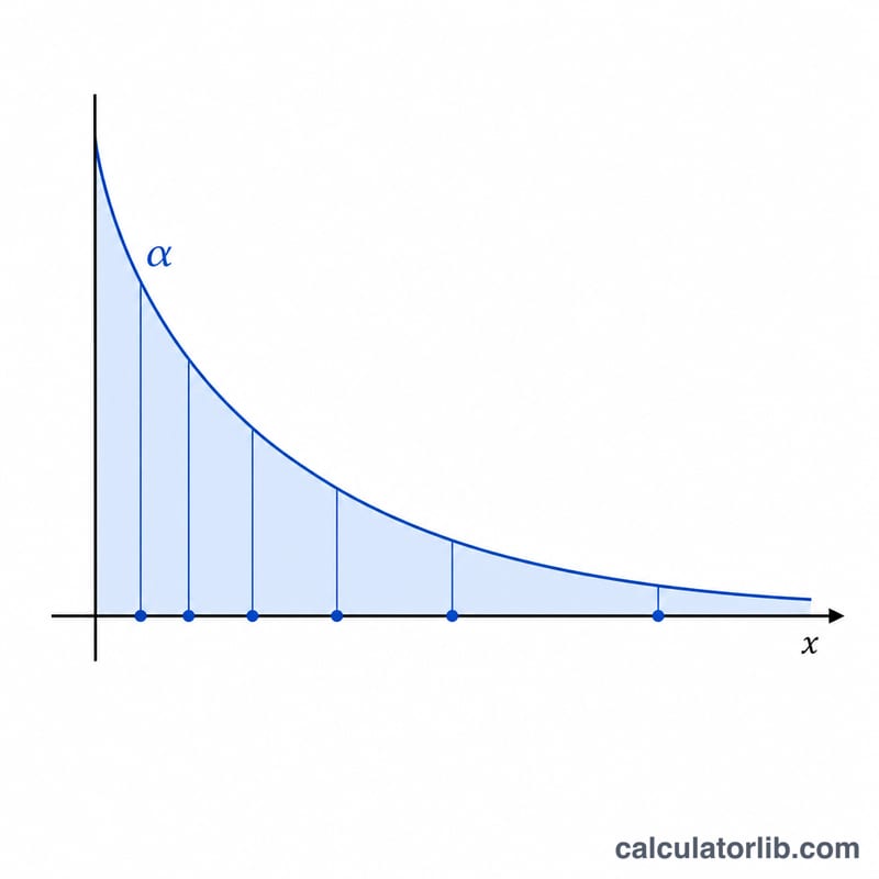
Gauss-Laguerre quadrature is a numerical method for approximating improper integrals over the semi-infinite interval (0, infinity) whose integrand decays like an exponential. It replaces the integral with a weighted sum evaluated at carefully chosen sample points called nodes. For a chosen order \(n\) the rule is exact for any polynomial of degree up to \(2n-1\) (against the weight \(x^{\alpha} e^{-x}\)), which makes it remarkably accurate for smooth integrands using only a handful of evaluations.
How to use this calculator
First pick an input mode. Choose f(x) if your integral already has the form integral of \(x^{\alpha} e^{-x} f(x)\, dx\) and you only want to type the factor \(f\). Choose g(x) if you have a complete integrand \(g(x)\) over (0, infinity); the tool then divides out the built-in weight automatically. Enter the function in the variable \(x\) using standard notation (+, -, *, /, ^, sqrt, exp, ln, sin, cos, tan, etc.), set the number of nodes \(n\), and set the weight parameter \(\alpha\) (use 0 for ordinary Gauss-Laguerre). Increasing \(n\) improves accuracy for smooth functions.
The formula explained
The nodes \(x_i\) are the roots of the generalized Laguerre polynomial \(L_n^{(\alpha)}(x)\), and the weights \(w_i\) are obtained by the Golub-Welsch algorithm: the eigenvalues of a symmetric tridiagonal Jacobi matrix give the nodes, while \(w_i = \Gamma(\alpha+1)\) times the square of the first component of each normalized eigenvector. The integral is then approximated by the weighted sum shown above.
$$\int_{0}^{\infty} x^{\alpha} e^{-x}\, g(x)\, dx \approx \sum_{i=1}^{n} w_i\, g(x_i)$$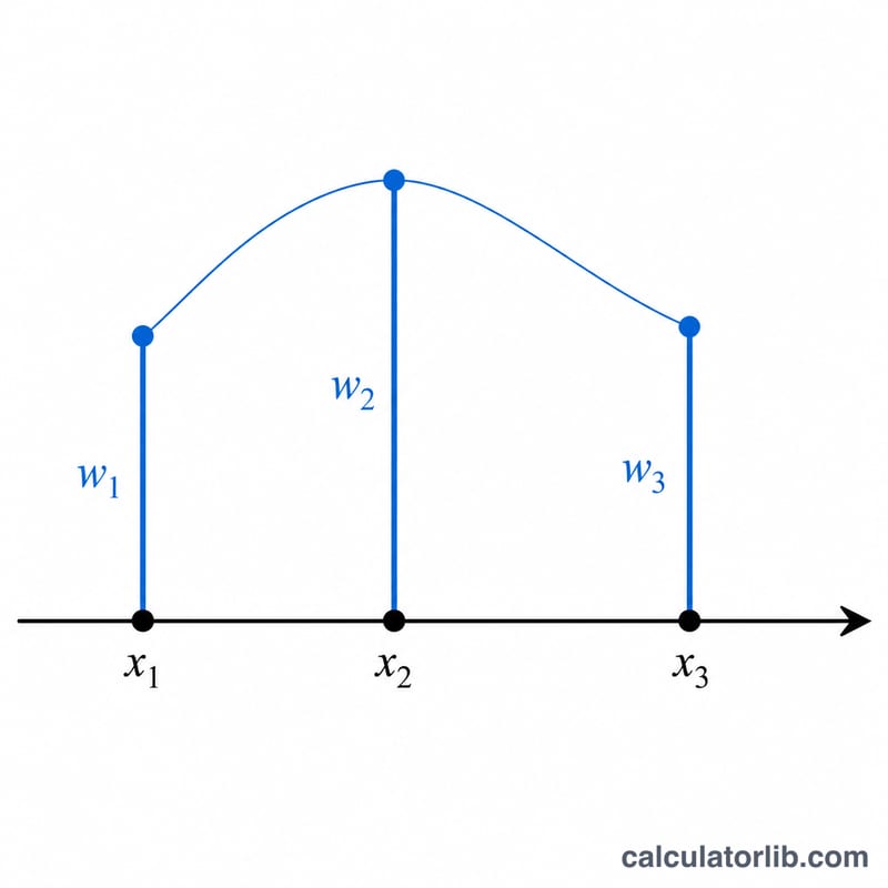
Worked example
Take \(\alpha = 0\), \(n = 2\), mode f(x), \(f(x) = x^2\) (so we estimate integral of \(x^2 e^{-x}\, dx\), whose exact value is \(\Gamma(3) = 2\)). The two nodes are \(x_1 = 2 - \sqrt{2} = 0.585786\) with \(w_1 = 0.853553\), and \(x_2 = 2 + \sqrt{2} = 3.414214\) with \(w_2 = 0.146447\). The sum is $$0.853553 \times 0.343146 + 0.146447 \times 11.656854 = 0.292893 + 1.707107 = 2.000000,$$ matching the exact answer exactly because \(x^2\) is a polynomial of degree \(2 \le 2n-1 = 3\).
FAQ
What does the parameter alpha do? It sets the exponent in the weight \(x^{\alpha} e^{-x}\). Use \(\alpha = 0\) for standard Gauss-Laguerre. Values must satisfy \(\alpha > -1\) so the weight remains integrable.
Why is my result inaccurate? Either the integrand is not smooth or it does not decay fast enough on (0, infinity). The rule always returns a finite number, but it is only meaningful when the true integral converges and the integrand is well approximated by polynomials times the weight. Increase \(n\) to test convergence.
What is the difference between f and g modes? In f mode you supply only the factor multiplying the built-in weight; in g mode you supply the entire integrand and the weight is removed inside the sum. Both give the same answer when set up consistently.