What is Gauss-Hermite quadrature?
Gauss-Hermite quadrature is a numerical integration method for integrals over the entire real line, from minus infinity to plus infinity. It is built around the Gaussian weight function \(e^{-x^{2}}\) and is exact for any polynomial of degree up to \(2n-1\) (in the weight-removed sense). Because it is pure mathematics, the rule is identical in every country and unit system. It is widely used in physics, statistics (expectations under a normal distribution), and engineering.
How to use this calculator
Pick an integrand form. Choose g(x) if you are entering the complete function you want to integrate over (-inf, inf); choose f(x) if you have already factored out the \(e^{-x^{2}}\) weight. Type the expression in the variable x (you can use exp, log, sqrt, sin, cos, tan, sinh, cosh, abs, pi, e, ^, and the usual operators). Finally set the number of nodes \(n\). More nodes give higher accuracy for smooth, Gaussian-like integrands; values of 8 to 30 are typical.
The formula explained
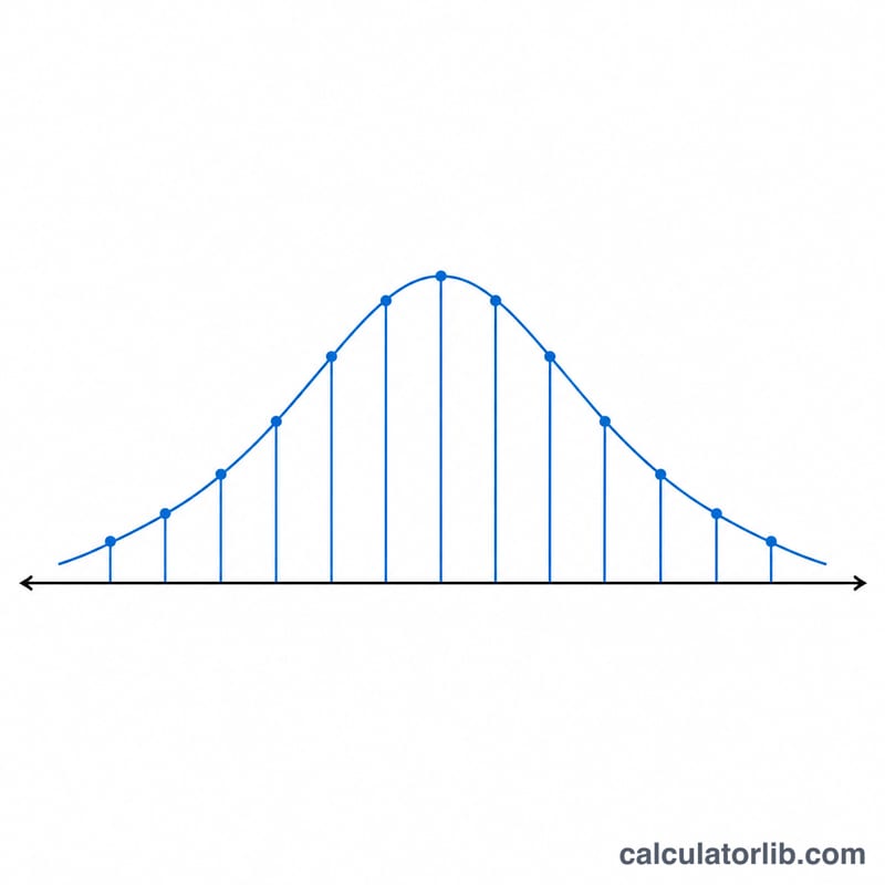
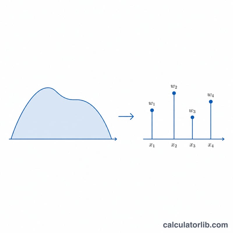
The method evaluates the integrand at the \(n\) roots \(x_i\) of the physicists' Hermite polynomial \(H_n(x)\) and combines them with weights $$w_i = \frac{2^{n-1}\, n!\, \sqrt{\pi}}{n^{2}\,[H_{n-1}(x_i)]^{2}}.$$ In f-mode the estimate is $$\int_{-\infty}^{\infty} f(x)\,dx \;\approx\; \sum_{i=1}^{n} w_i\, e^{x_i^{2}}\,f(x_i).$$ In g-mode the weight is divided back out using the modified weight \(W_i = w_i\, e^{x_i^{2}}\), giving $$\int_{-\infty}^{\infty} e^{-x^{2}}\,g(x)\,dx \;\approx\; \sum_{i=1}^{n} w_i\, e^{x_i^{2}}\,g(x_i).$$ The nodes and weights here are produced by the numerically stable Golub-Welsch algorithm, which finds them as eigenvalues and eigenvectors of a symmetric tridiagonal Jacobi matrix.
Worked example
Take f-mode with \(f(x) = 1\) and \(n = 2\). The two nodes are \(x = \pm \frac{1}{\sqrt{2}}\) with equal weights \(w = \frac{\sqrt{\pi}}{2} = 0.8862269255\). The sum is $$0.8862269255 + 0.8862269255 = 1.7724538509,$$ which equals \(\sqrt{\pi}\) exactly, the true value of the integral of \(e^{-x^{2}}\) over the real line. Equivalently, in g-mode with \(g(x) = \exp(-x^{2})\) and \(n = 2\), the modified weights recover the same answer, \(1.7724538509\).
FAQ
When does it converge slowly? When the integrand is not well approximated by \(e^{-x^{2}}\) times a polynomial, for example functions with slow polynomial decay, fat tails, or singularities on the real axis. Increase \(n\) or use a different method.
What does the \(e^{x_i^{2}}\) factor do in g-mode? It cancels the built-in Gaussian weight so you can supply the full integrand. For outer nodes it can become large, so \(g(x)\) should decay at least as fast as \(e^{-x^{2}}\) for good results.
Is the rule exact for polynomials? Yes, in f-mode it integrates any polynomial of degree up to \(2n-1\) exactly.