Gauss-Legendre Numerical Integration (Quadrature) Calculator

Enter Calculation

f(x)

Lower limit a

Upper limit b

Number of points n 2 3 4 5 6 7 8 9 10 11 12 13 14 15 16 17 18 19 20 21 22 23 24 25 26 27 28 29 30 31 32 33 34 35 36 37 38 39 40 41 42 43 44 45 46 47 48 49 50 51 52 53 54 55 56 57 58 59 60 61 62 63 64 65

Results

Integral of f(x) from a to b (approximate)

3.1415926536

n-point Gauss-Legendre quadrature

Lower limit a	0
Upper limit b	1
Points n	20
Exact for polynomials up to degree	2n − 1

What is Gauss-Legendre quadrature?

Gauss-Legendre quadrature is a numerical method for estimating a definite integral. Instead of slicing the interval into many equal strips, it evaluates the integrand at a small number of cleverly chosen points (the nodes) and combines them with carefully tuned weights. The payoff is remarkable accuracy: an n-point Gauss-Legendre rule integrates any polynomial up to degree \(2n - 1\) exactly, and gives excellent results for smooth functions with far fewer evaluations than the trapezoidal or Simpson rules.

Gauss-Legendre quadrature approximates the area under f(x) using cleverly chosen sample points and weights.

How to use this calculator

Enter the integrand as an expression in x (for example 4/(1+x^2), sin(x)*exp(-x), or sqrt(1-x^2)). Set the lower limit a and upper limit b, then pick the number of points n from 2 to 64. Higher n gives more accuracy for smooth integrands. Supported operators are + - * / ^; supported functions include sin, cos, tan, asin, acos, atan, sinh, cosh, tanh, exp, log/ln, log10, sqrt and abs, plus the constants pi and e.

The formula explained

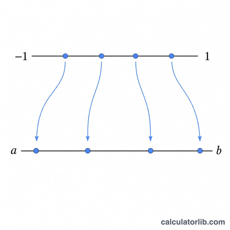
The classic rule is defined on the interval [-1, 1]: the integral is approximated by the weighted sum of f at the Legendre roots \(x_i\). To handle a general interval [a, b], a linear change of variable maps t in [-1, 1] to \(x = \frac{b-a}{2}t + \frac{b+a}{2}\), with \(dx = \frac{b-a}{2}\,dt\).

$$\int_{a}^{b} f(x)\,dx \approx \frac{b-a}{2}\sum_{i=1}^{n} w_i\,f\!\left(\frac{b-a}{2}x_i + \frac{a+b}{2}\right)$$

This calculator computes the nodes on the fly using Newton's method on the Legendre polynomial recurrence, so no lookup table is needed.

The standard nodes on [-1, 1] are linearly mapped onto the integration interval [a, b].

Worked example

Take \(f(x) = \frac{4}{1 + x^2}\) on [0, 1], whose exact integral is \(\pi\). With \(n = 2\) the nodes are \(\pm\frac{1}{\sqrt{3}}\) with weights 1 and 1. Mapping them into [0, 1] and evaluating gives \(f(0.2113) = 3.8290\) and \(f(0.7887) = 2.4661\); the sum times the scale 0.5 yields about 3.1476 - already close to \(\pi\) after just two evaluations. With \(n = 20\) the result matches \(\pi\) to roughly \(3.14159265359\).

FAQ

What happens if a = b? The interval has zero width, so the integral is exactly 0.

Can b be less than a? Yes. The rule returns the signed result, consistent with the convention that reversing the limits negates the integral.

Why might the result look wrong? Gauss-Legendre assumes the integrand is finite at every node. An interior singularity (a division by zero or a log of a negative number) can produce a meaningless value; the calculator warns you when a node yields NaN or infinity. Note that endpoints a and b themselves are never evaluated, which helps with mild endpoint behavior.