What this calculator does
This tool computes the nodes (abscissae \(x_i\)) and weights \(w_i\) for the classical Gaussian quadrature rules. With these you approximate a weighted integral as a finite weighted sum, integrating polynomials up to degree \(2n-1\) exactly for the standard Gauss rules. Supported rules: Gauss-Legendre, Chebyshev of the first and second kind, generalized Laguerre, Hermite, Jacobi, and Gauss-Lobatto.
$$\int_{-1}^{1} f(x)\,dx \approx \sum_{i=1}^{\text{n}} w_i\, f(x_i), \qquad \text{Gauss-Legendre}$$How to use it
Pick a rule under "Kinds", choose the order \(n\) (number of nodes, 2 to 100), and for Laguerre or Jacobi supply the exponent parameters Alpha and Beta (each must be greater than \(-1\)). The result lists each node and its weight, plus the sum of weights, which should equal the 0th moment of the weight function (for Legendre that is 2, for Hermite it is the square root of pi).
The formula explained
For a family of orthogonal polynomials with three-term recurrence, the nodes are the roots of the degree-\(n\) polynomial and the weights come from the eigenvectors of the symmetric tridiagonal Jacobi matrix \(J\) (the Golub-Welsch method): \(w_i = \mu_0 (v_{1,i})^2\). Chebyshev rules use exact trigonometric closed forms, Legendre and Lobatto use Newton iteration on the Legendre polynomial, and Laguerre, Hermite and Jacobi use the Jacobi-matrix eigensolver.
$$w_i = \frac{2}{\left(1-x_i^2\right)\left[P_{\text{n}}^{\prime}(x_i)\right]^2}$$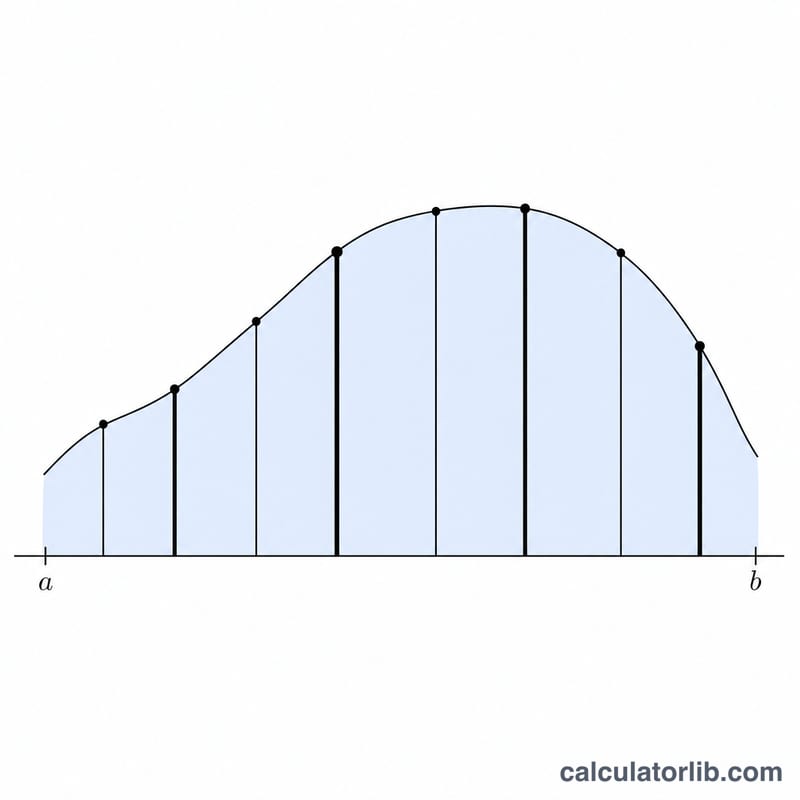
Worked example
Gauss-Legendre with \(n = 2\): nodes are plus and minus \(1/\sqrt{3} = 0.5773502692\), and both weights equal 1, so the sum of weights is 2. Check: the integral of \(x^2\) over \([-1, 1]\) is \(2/3\), and the rule gives $$1\cdot\left(\tfrac{1}{3}\right) + 1\cdot\left(\tfrac{1}{3}\right) = \tfrac{2}{3}.$$
![Symmetric Gauss-Legendre nodes on [-1,1] with weight bars tallest at the center](https://cdn.calculatorlib.com/v5/calculators/inline-2-3af7a8df1c/gauss-quadrature-nodes-weights-calculator.png)
FAQ
Why should weights be positive? For classical Gauss rules all weights are strictly positive; a negative weight signals numerical error.
What does the sum of weights mean? It equals the integral of the weight function over the interval (the 0th moment). For Hermite, \(e^{-x^2}\) integrates to \(\sqrt{\pi}\) over the whole line.
Why must Alpha and Beta exceed -1? Otherwise the weight function is not integrable and the moments diverge, so no valid rule exists.


