What is the Gaussian Quadrature Calculator?
This is a pure-mathematics tool (it works identically in every country) that numerically approximates a definite integral using a Gaussian-quadrature rule you choose. Gaussian quadrature evaluates the integrand at a small set of cleverly chosen points called nodes, multiplies each value by a matching weight, and adds them up. With \(n\) points it integrates polynomials up to degree \(2n-1\) exactly, which makes it far more accurate than equally-spaced methods like the trapezoid or Simpson rules for smooth functions.
How to use it
Pick a quadrature method, set the number of points \(n\), type the integrand \(f(x)\) using standard syntax (+ - * / ^, parentheses, sin, cos, tan, exp, log, ln, sqrt, abs, pi, e), and for the finite rules supply the limits \(a\) and \(b\). The weight function \(w(x)\) is built into each rule, so enter only the smooth part \(f(x)\): for Gauss-Laguerre omit the \(x^{\alpha} e^{-x}\) factor, for Gauss-Hermite omit \(e^{-x^2}\), and for Chebyshev/Jacobi omit the \((1-x^2)\) weight. The Significant digits dropdown changes only how many digits are displayed.
The formula
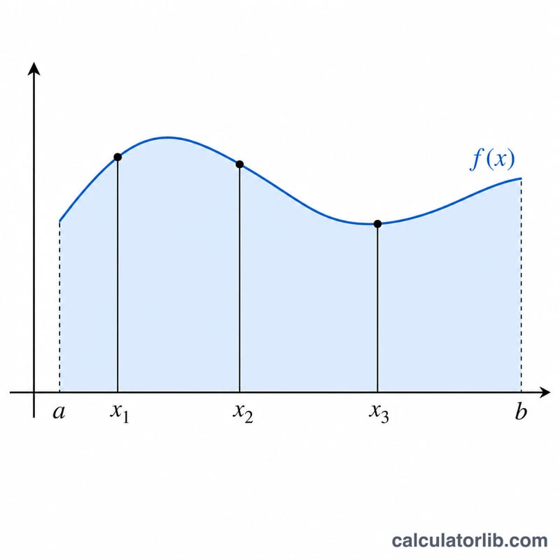
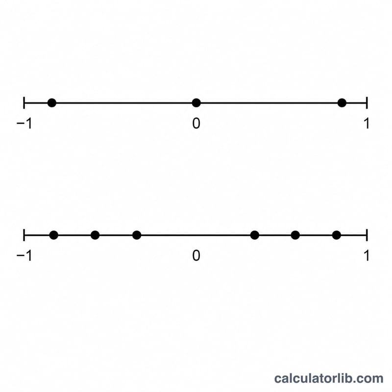
Every rule has the same shape: the integral of \(w(x) f(x)\) over the canonical interval is approximated by the sum of \(w_i\) times \(f(x_i)\), where the nodes \(x_i\) are roots of the relevant orthogonal polynomial and \(w_i\) are the Golub-Welsch weights. For a finite arbitrary interval \([a,b]\) with weight 1, the canonical nodes \(t_i\) in \([-1,1]\) are mapped by $$x_i = \frac{b-a}{2} t_i + \frac{a+b}{2}$$ and the whole sum is scaled by \(\frac{b-a}{2}\). $$\int_{a}^{b} f(x)\,dx \approx \frac{b-a}{2}\sum_{i=1}^{n} w_i\, f\!\left(\frac{b-a}{2}x_i + \frac{a+b}{2}\right)$$
Worked example
Choose Gauss-Legendre, \(n=20\), \(f(x)=\frac{4}{1+x^2}\), \(a=0\), \(b=1\). The exact value is $$4\arctan(1) = \pi = 3.14159265358979.$$ The 20-point Legendre rule maps the nodes into \([0,1]\), scales the weights by \(\frac{1}{2}\), and returns \(3.141592653589793\) - agreeing with \(\pi\) to full double precision. That is why \(\frac{4}{1+x^2}\) is the default integrand.
FAQ
Why does my answer look wrong for Laguerre or Hermite? Those rules already include the \(e^{-x}\) or \(e^{-x^2}\) weight; enter only the remaining factor, not the full integrand. For example to get the integral of \(e^{-x^2}\) over the whole line, set \(f(x)=1\), which gives \(\sqrt{\pi}\).
What do alpha and beta do? \(\alpha\) is the exponent in the Laguerre \(x^{\alpha}\) weight and one Jacobi exponent; \(\beta\) is the other Jacobi exponent. Both must exceed \(-1\) or the weight integral diverges.
Does more points always help? For smooth functions higher \(n\) improves accuracy, but for functions with singularities or sharp peaks inside the interval it can hurt. Increase \(n\) gradually and watch for convergence.