What Is a Differential Equation Calculator?
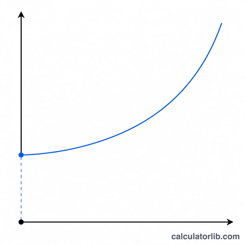
A differential equation (Differentialgleichung) relates a function to its own rate of change. This calculator focuses on the classic first-order linear equation \( \frac{dy}{dx} = k\,y \), which models exponential growth and decay in physics, biology, finance, and engineering. It returns both the exact solution and a numerical approximation so you can compare theory with computation.
The Formula Explained
With an initial condition \( y(x_0) = y_0 \), the equation has the closed-form solution shown below, where \(y_0\) is the starting value, \(k\) is the rate constant, and \(x\) is the target point.
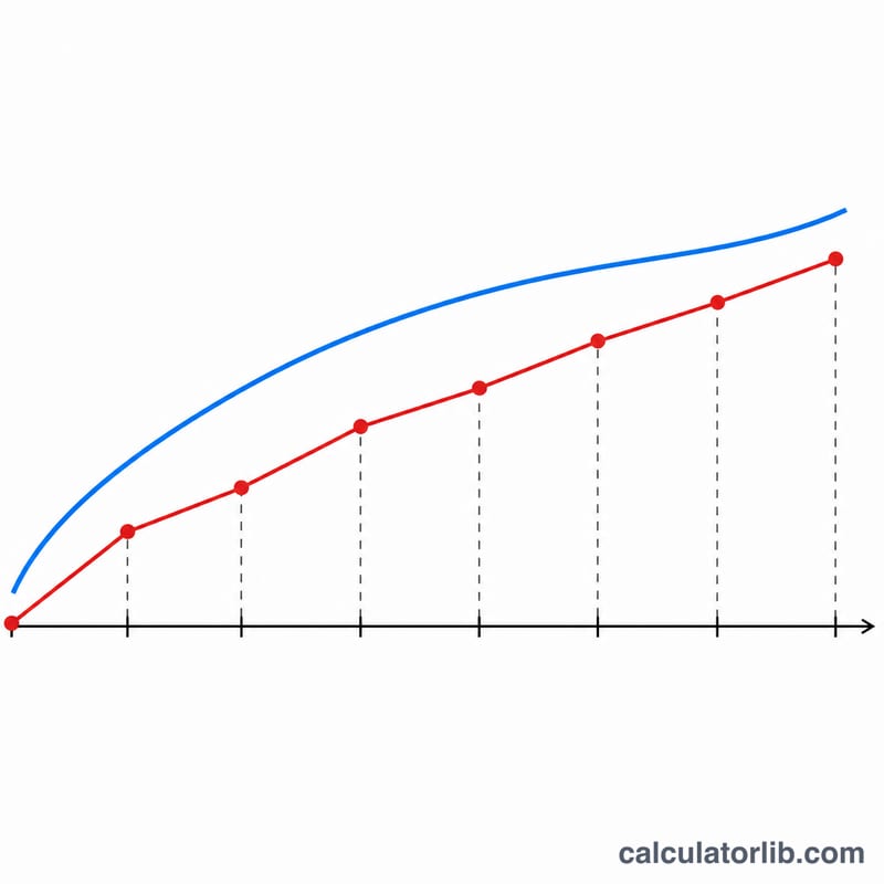
$$y(x) = y_0\,e^{k(x - x_0)}$$When a closed form is hard to obtain, the Euler method steps forward in small increments \(h = \frac{x - x_0}{n}\) using \( y_{i+1} = y_i + h\,k\,y_i \). Smaller steps (larger \(n\)) reduce the approximation error.
How to Use It
Enter the initial value \(y_0\), the rate constant \(k\), the start point \(x_0\), the target \(x\), and the number of Euler steps \(n\). The calculator reports the exact value, the Euler estimate, the step size, and the absolute error between them.
Worked Example
Take \(y_0 = 1\), \(k = 1\), \(x_0 = 0\), \(x = 1\) with one Euler step. The exact answer is
$$y(1) = 1\cdot e^{1\cdot(1-0)} = e \approx 2.71828$$The single Euler step gives \( y_1 = 1 + 1\times 1\times 1 = 2 \), so the absolute error is about \(0.718\). Using more steps drives the estimate toward \(e\).
More Worked Examples
All examples below use the first-order linear ODE \(\frac{dy}{dx} = k y\). Its exact closed-form solution is \(y(x) = y_0\,e^{k(x - x_0)}\), and the explicit (forward) Euler approximation uses a fixed step size \(h = \frac{x - x_0}{n}\) with the update rule \(y_{i+1} = y_i + h\,k\,y_i\). These are general mathematical results, not tied to any country or standard.
Example 1 — Exponential decay (exact)
Inputs: \(y_0 = 100\), \(k = -0.5\), \(x_0 = 0\), \(x = 2\). Because \(k<0\) the quantity decays. Substituting into the exact solution:
$$y(2) = 100 \cdot e^{-0.5\,(2 - 0)} = 100\,e^{-1} = 100 \cdot 0.367879 \approx 36.7879$$So the exact value is 36.7879.
Example 2 — Euler method, growth, n = 4
Inputs: \(y_0 = 100\), \(k = 0.5\), \(x_0 = 0\), \(x = 2\), \(n = 4\). Step size \(h = \frac{2 - 0}{4} = 0.5\). Each iteration multiplies by \((1 + hk) = (1 + 0.5 \cdot 0.5) = 1.25\):
- \(y_1 = 100 + 0.5 \cdot 0.5 \cdot 100 = 100 + 25 = 125\)
- \(y_2 = 125 + 0.5 \cdot 0.5 \cdot 125 = 125 + 31.25 = 156.25\)
- \(y_3 = 156.25 + 0.5 \cdot 0.5 \cdot 156.25 = 156.25 + 39.0625 = 195.3125\)
- \(y_4 = 195.3125 + 0.5 \cdot 0.5 \cdot 195.3125 = 195.3125 + 48.828125 = 244.140625\)
| Step \(i\) | \(x_i\) | \(y_i\) (Euler) |
|---|---|---|
| 0 | 0.0 | 100.000000 |
| 1 | 0.5 | 125.000000 |
| 2 | 1.0 | 156.250000 |
| 3 | 1.5 | 195.312500 |
| 4 | 2.0 | 244.140625 |
Exact value: \(y(2) = 100\,e^{0.5 \cdot 2} = 100\,e^{1} \approx 271.8282\). Absolute error: \(|271.8282 - 244.1406| \approx 27.6876\). Forward Euler underestimates a convex growth curve, so a larger \(n\) is needed to close this gap.
Example 3 — Euler method, decay, n = 4
Inputs: \(y_0 = 100\), \(k = -0.5\), \(x_0 = 0\), \(x = 2\), \(n = 4\). Step size \(h = 0.5\); each iteration multiplies by \((1 + hk) = (1 + 0.5 \cdot (-0.5)) = 0.75\):
- \(y_1 = 100 + 0.5 \cdot (-0.5) \cdot 100 = 100 - 25 = 75\)
- \(y_2 = 75 + 0.5 \cdot (-0.5) \cdot 75 = 75 - 18.75 = 56.25\)
- \(y_3 = 56.25 - 14.0625 = 42.1875\)
- \(y_4 = 42.1875 - 10.546875 = 31.640625\)
Exact value (from Example 1): \(y(2) \approx 36.7879\). Absolute error: \(|36.7879 - 31.6406| \approx 5.1473\). The error is much smaller than in the growth case because a decaying, concave curve is easier for Euler to track at the same step size.
FAQ
What order of equation does this solve? A first-order linear ODE of the form \( \frac{dy}{dx} = k\,y \).
Why does the Euler result differ from the exact value? Euler method is a first-order approximation; each step introduces truncation error that shrinks as \(n\) grows.
Can k be negative? Yes. A negative \(k\) models exponential decay, such as radioactive half-life or cooling.