
What is the Lotka-Volterra model?
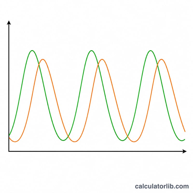
The Lotka-Volterra equations are a pair of first-order nonlinear differential equations that describe the dynamics of biological systems in which two species interact — one as predator and one as prey. Independently derived by Alfred Lotka and Vito Volterra in the 1920s, the model captures the cyclic rise and fall of populations: prey multiply, predators feast and grow, prey crash, predators starve, and the cycle repeats.
How to use this calculator
Enter the initial prey population (\(x_0\)) and predator population (\(y_0\)), the four rate parameters (\(\alpha\) prey growth, \(\beta\) predation, \(\delta\) predator growth from eating prey, \(\gamma\) predator death), a time step (\(dt\)), and the number of steps to integrate. The calculator advances the system using the classic fourth-order Runge-Kutta (RK4) method and reports the final populations, the peak each population reached, and the analytic equilibrium point.
The formula explained
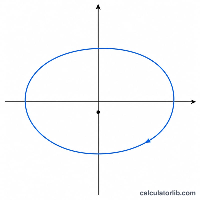
The prey equation \(\frac{dx}{dt} = \alpha x - \beta x y\) says prey grow exponentially but are removed when they meet predators. The predator equation \(\frac{dy}{dt} = \delta x y - \gamma y\) says predators grow from successful hunts and die off naturally. The nonzero equilibrium sits at $$x^{*} = \frac{\gamma}{\delta} \qquad y^{*} = \frac{\alpha}{\beta}$$ — at that point both derivatives are zero and the populations remain constant.
Worked example
With \(x_0 = 40\), \(y_0 = 9\), \(\alpha = 0.1\), \(\beta = 0.02\), \(\delta = 0.01\), \(\gamma = 0.1\), \(dt = 0.1\) over 1000 steps (\(t\) up to 100), the populations oscillate. The equilibrium is $$x^{*} = \frac{0.1}{0.01} = 10 \text{ prey} \qquad y^{*} = \frac{0.1}{0.02} = 5 \text{ predators}$$ the center around which the cycle orbits.
FAQ
What integration method is used? The fourth-order Runge-Kutta method, which is far more accurate than simple Euler stepping for the same step size.
Why does my population blow up or hit zero? Very large time steps or extreme rates can make the numerical solution unstable. Reduce \(dt\) for smoother, more accurate cycles.
What if I start at the equilibrium? If \(x_0 = \frac{\gamma}{\delta}\) and \(y_0 = \frac{\alpha}{\beta}\), both derivatives are zero so the populations stay constant — a fixed point of the system.