What this calculator does
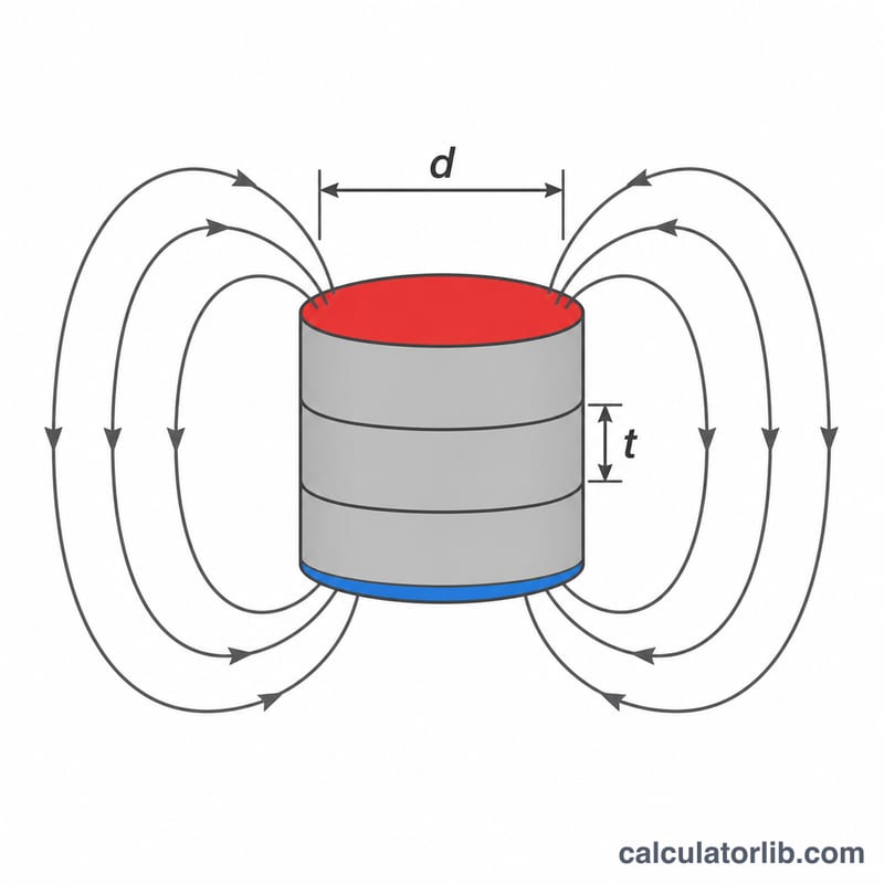
Stacking identical disc or cylinder magnets with their poles aligned makes one longer magnet. The surface gauss at the end face rises, but not in a simple multiple: the field grows more slowly as the stack gets longer compared with its diameter. This calculator estimates the combined surface field from the gauss rating of one magnet, its diameter, its thickness and the number stacked.
How to use it
Enter the surface gauss rating of a single magnet, the number of magnets in the stack, the diameter and the thickness of each magnet in millimetres. The result shows the combined gauss, the multiplier compared with a single magnet, the field in tesla, the stack length and the implied material remanence.
The formula explained
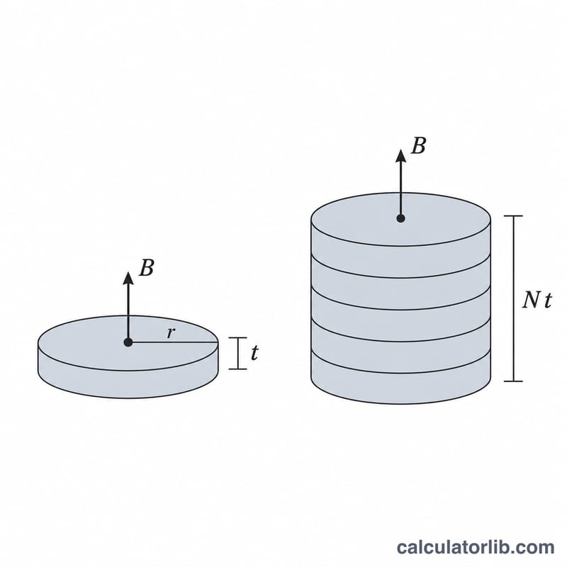
For an axially magnetized cylinder of length \(L\) and radius \(R\), the on-axis field at the centre of the end face is:
$$B = \frac{B_r}{2}\cdot\frac{L}{\sqrt{R^2+L^2}}$$Using the single-magnet rating to eliminate \(B_r\) gives the stacked field for \(n\) magnets of thickness \(t\):
$$B_n = B_1 \times \frac{n\sqrt{R^2+t^2}}{\sqrt{R^2+n^2 t^2}}$$Here \(B_1\) is the single-magnet gauss, \(R\) is the radius and \(t\) is the thickness of one magnet. As \(n\) grows, \(B_n\) approaches \(B_r/2\).
Worked example
Two magnets rated 3000 G, diameter 20 mm (\(R = 10\) mm), thickness 5 mm each:
$$B_2 = 3000 \times \frac{2\sqrt{100+25}}{\sqrt{100+100}} = 3000 \times \frac{22.36}{14.142} \approx 4743\,\text{G}$$Stacking two magnets therefore gives about 1.58 times the field, not 2 times.
Stacked Gauss for Different Magnet Counts and Aspect Ratios
All rows use the same single-magnet rating of B1 = 3000 G and the stacking formula \(B_n = B_1 \cdot \dfrac{n\sqrt{R^2+t^2}}{\sqrt{R^2+n^2t^2}}\), where \(R\) is the disc radius (diameter ÷ 2), \(t\) is the thickness of one disc and \(n\) is the number of discs. The 3000 G figure is illustrative, chosen so the shapes can be compared directly.
Example substitution (20 mm × 5 mm, n = 5, so R = 10 mm, t = 5 mm): \(B_5 = 3000 \cdot \dfrac{5\sqrt{100+25}}{\sqrt{100+625}} = 3000 \cdot \dfrac{55.902}{26.926} \approx\) 6228 G.
| Stack size n | Thin-wide: 20 mm dia × 3 mm Combined G (multiplier) |
Example: 20 mm dia × 5 mm Combined G (multiplier) |
Thick-narrow: 10 mm dia × 10 mm Combined G (multiplier) |
|---|---|---|---|
| 1 | 3000 (1.000×) | 3000 (1.000×) | 3000 (1.000×) |
| 2 | 5371 (1.790×) | 4743 (1.581×) | 3254 (1.085×) |
| 3 | 6984 (2.328×) | 5582 (1.861×) | 3308 (1.103×) |
| 5 | 8687 (2.896×) | 6228 (2.076×) | 3337 (1.112×) |
| 10 | 9905 (3.302×) | 6578 (2.193×) | 3350 (1.117×) |
| Limit as n → ∞ | 10,440 (3.480×) | 6708 (2.236×) | 3354 (1.118×) |
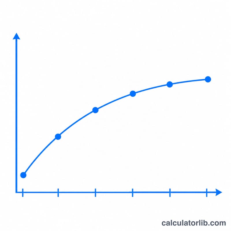
The limit follows because for large n the term \(n^2t^2\) dominates, so \(B_n \to B_1\sqrt{R^2+t^2}\,/\,t\). Thin, wide discs gain the most from stacking. Thick, narrow discs are already close to the limit with a single magnet, so extra discs add very little.
Interpreting Your Result
The calculator gives an idealised on-axis surface field: the field at the center of the end face of the stack, along the magnetization axis. It is not the average over the face, and it is not the field at some distance from the surface. Off-center or farther from the face, the field is lower and falls off quickly.
For a single uniformly magnetized disc, the on-axis surface field is \(B_1 = \dfrac{B_r}{2}\cdot\dfrac{t}{\sqrt{R^2+t^2}}\). As the stack grows, the multiplier \(B_n/B_1\) approaches \(\sqrt{R^2+t^2}\,/\,t\), so the stacked field approaches \(B_r/2\). Dividing \(B_r/2\) by \(B_1\) gives that limiting multiplier. For example, a 20 mm × 5 mm disc has a limit of 2.236×, and no stack of that shape can exceed it, however many discs you add.
Compare the multiplier with n. If it is well below n, you are in the region of diminishing returns: each additional disc raises the field by less than the previous one. In the table above, ten 10 mm × 10 mm discs give only 1.117× the field of one disc.
Real measurements will differ from the calculated number. A gaussmeter reading depends on the probe distance (the sensing element sits slightly inside the probe housing), on its position over the face, and on its orientation. Actual magnets also vary in grade and tolerance. The units convert as 10,000 G = 1 T, so 6228 G is about 0.62 T.
Definitions and Glossary
- Gauss (G): the CGS unit of magnetic flux density. 1 G = 0.0001 T.
- Tesla (T): the SI unit of magnetic flux density. 1 T = 10,000 G.
- Surface field: the flux density measured at or very near the surface of a magnet, usually at the center of a pole face. It is much higher than the field some distance away.
- Remanence (Br): the flux density remaining in a magnetic material after the magnetizing field is removed. It is a material property that depends on the grade. For a long magnet, the surface field approaches Br/2.
- Axial magnetization: magnetization along the axis of the disc, so the north and south poles are on the two flat faces. This is the assumption in the stacking formula.
- Magnet grade: a label such as N42 for sintered neodymium (NdFeB) magnets. The number indicates the maximum energy product (in MGOe), and higher numbers generally mean higher remanence.
- On-axis field: the field along the line through the center of the disc, parallel to the magnetization direction.
- Aspect ratio (length to diameter): the magnetized length (stack height) divided by the diameter. A higher ratio means a stack closer to the Br/2 limit, so adding discs gives less benefit.
FAQ
Does stacking double the gauss?
No. Doubling the length of a magnet raises the surface field only by a factor less than 2, and thin wide magnets gain the most.
Does this predict pull force?
Not directly. Pull force depends on the surface field, contact area and the target material, and it is not proportional to gauss.
What about gaps or opposing poles?
This model assumes the magnets touch with matching poles. Gaps, mixed grades or opposing orientation will change the result, and the figures are an idealised estimate.