

什麼是判定係數(R²)?
判定係數通常寫作 \(R^{2}\),用來衡量模型的預測值與實際觀測資料的吻合程度。它代表依變數(被預測變數)中,能被模型解釋的變異比例。\(R^{2}\) 的最大值為 1,表示完美擬合,預測值與實際值完全相同;數值為 0 時,代表模型的表現與單純用平均數來預測沒有差別;當模型甚至比「直接用平均數」還差時,\(R^{2}\) 還會出現負值。
如何使用這個計算器
請依相同順序,分別輸入一組實際觀測值(y)與對應的預測值(ŷ),每組數字以逗號分隔。計算器會把兩組數值一一配對,先求出實際值的平均數,再計算殘差平方和(\(SS_{res}\))與總平方和(\(SS_{tot}\)),最後算出 \(R^{2}\) 以及模型可解釋的變異百分比。
公式說明
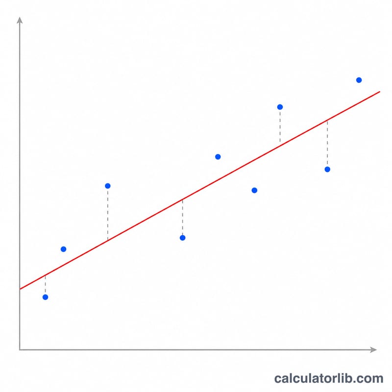
$$R^{2} = 1 - \frac{SS_{res}}{SS_{tot}}$$其中 \(SS_{res} = \sum (y_{i} - \hat{y}_{i})^{2}\),代表模型預測後仍殘留的誤差;\(SS_{tot} = \sum (y_{i} - \bar{y})^{2}\),則代表資料相對於自身平均數的總變異量。兩者相除,可看出模型「沒能解釋」的變異比例;再用 1 減去這個比例,就得到模型「成功解釋」的變異比例。
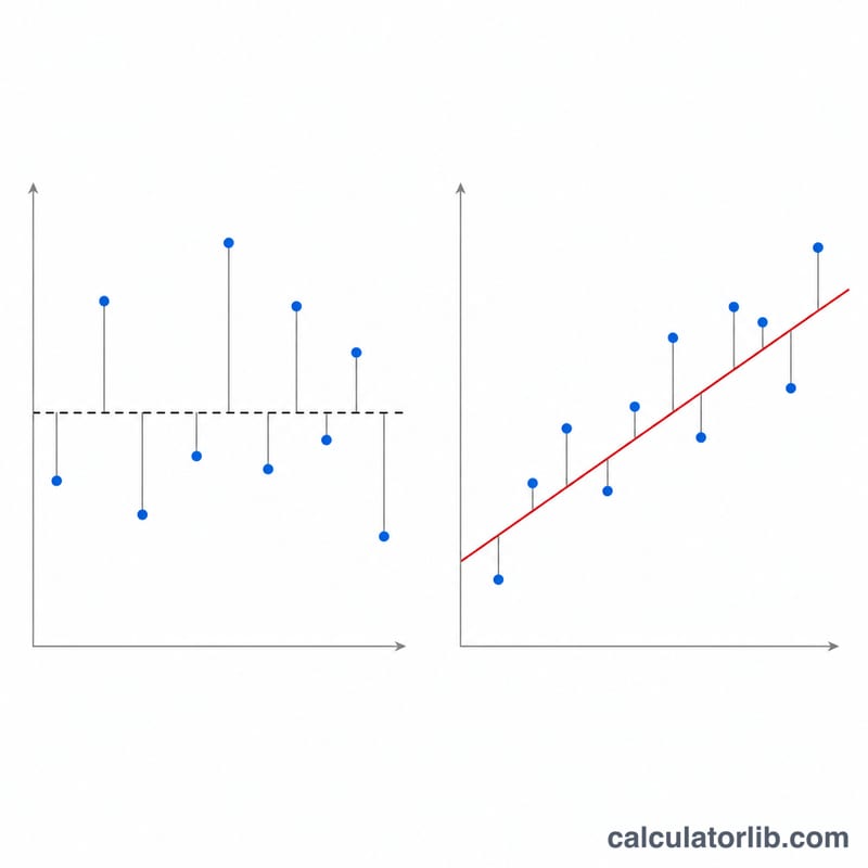
實例演算
實際值 = [3, −0.5, 2, 7],預測值 = [2.5, 0.0, 2, 8]。實際值的平均數 = 2.875。$$SS_{res} = 0.5^{2} + 0.5^{2} + 0^{2} + 1^{2} = 0.25 + 0.25 + 0 + 1 = 1.5$$ $$SS_{tot} = (0.125)^{2} + (3.375)^{2} + (0.875)^{2} + (4.125)^{2} \approx 0.0156 + 11.3906 + 0.7656 + 17.0156 = 29.1875$$ $$R^{2} = 1 - \frac{1.5}{29.1875} \approx 0.9486$$因此這個模型約可解釋 94.9% 的變異。
常見問題
\(R^{2}\) 會是負值嗎?會。如果你的預測結果比「每次都直接猜平均數」還要差,\(SS_{res}\) 就會大於 \(SS_{tot}\),\(R^{2}\) 便會變成負數。
\(R^{2}\) 高就代表模型好嗎?不一定。\(R^{2}\) 可能因為過度擬合(overfitting)或加入無關的預測變數而被「灌水」。建議搭配殘差圖以及樣本外(out-of-sample)的表現一起檢視。
\(R^{2}\) 和相關係數有什麼不同?在簡單線性迴歸中,\(R^{2}\) 等於實際值與預測值之間皮爾森相關係數(\(r\))的平方。