
What Is the Coefficient of Determination (R²)?
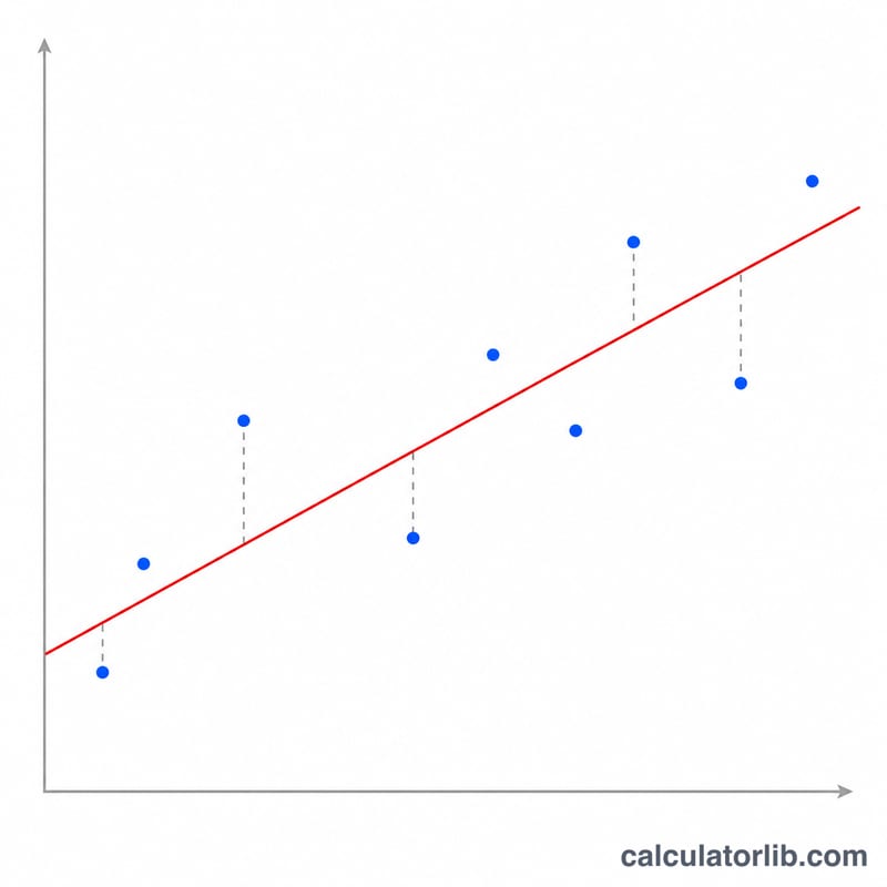
The coefficient of determination, written \(R^{2}\), measures how well a model's predictions match the actual observed data. It is the proportion of the variance in the dependent variable that is explained by the model. \(R^{2}\) ranges from 1 (a perfect fit, where predictions exactly equal actual values) down through 0 (the model is no better than simply predicting the mean) and can even go negative when a model performs worse than the mean baseline.
How to Use This Calculator
Enter your list of actual observed values (y) and the matching list of predicted values (ŷ), each as comma-separated numbers in the same order. The calculator pairs them up, computes the mean of the actual values, then derives the residual sum of squares (SSres) and the total sum of squares (SStot) to return \(R^{2}\) and the percent of variance explained.
The Formula Explained
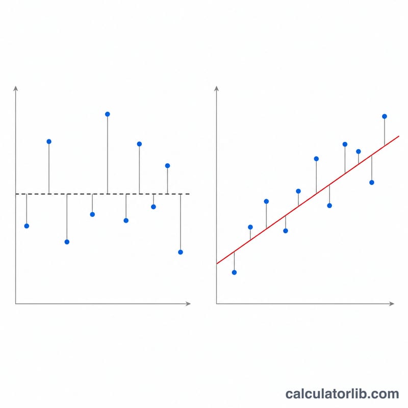
$$R^{2} = 1 - \frac{SS_{res}}{SS_{tot}}$$ Here \(SS_{res} = \sum (y_i - \hat{y}_i)^{2}\) captures the error left over after the model's predictions, while \(SS_{tot} = \sum (y_i - \bar{y})^{2}\) captures the total variability of the data around its own mean. Dividing one by the other tells you what fraction of variability the model failed to explain; subtracting from 1 gives the fraction it did explain.
Worked Example
Actual = [3, −0.5, 2, 7], Predicted = [2.5, 0.0, 2, 8]. Mean of actual = 2.875. $$SS_{res} = 0.5^{2} + 0.5^{2} + 0^{2} + 1^{2} = 0.25 + 0.25 + 0 + 1 = 1.5$$ $$SS_{tot} = (0.125)^{2} + (3.375)^{2} + (0.875)^{2} + (4.125)^{2} \approx 0.0156 + 11.3906 + 0.7656 + 17.0156 = 29.1875$$ $$R^{2} = 1 - \frac{1.5}{29.1875} \approx 0.9486$$ so the model explains about 94.9% of the variance.
FAQ
Can R² be negative? Yes. If your predictions are worse than just guessing the mean every time, \(SS_{res}\) exceeds \(SS_{tot}\) and \(R^{2}\) becomes negative.
Does a high R² mean a good model? Not always — \(R^{2}\) can be inflated by overfitting or by adding irrelevant predictors. Always check it alongside residual plots and out-of-sample performance.
What is the difference between R² and correlation? For simple linear regression, \(R^{2}\) equals the square of the Pearson correlation coefficient (\(r\)) between actual and predicted values.