What Is Friction Head Loss?
When water flows through a pipe, friction between the fluid and the pipe wall dissipates energy, producing a pressure drop known as friction head loss. This calculator estimates that loss using the Hazen-Williams equation, a widely used empirical formula for water in pressurized pipes at ordinary temperatures.
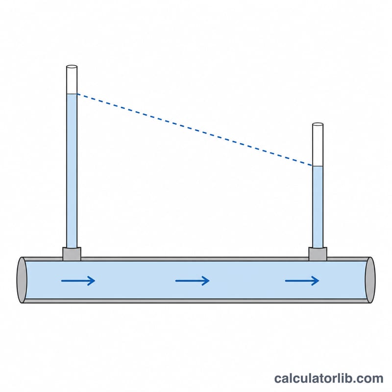
The Formula
The head loss \(h_f\) in meters is:
$$h_f = \frac{10.67\,L\,Q^{1.852}}{C^{1.852}\,D^{4.8704}}$$where \(L\) = pipe length in meters, \(Q\) = flow rate in cubic meters per second, \(D\) = internal diameter in meters, and \(C\) = the Hazen-Williams roughness coefficient (about 130 for new steel or plastic, 100 for older pipe).
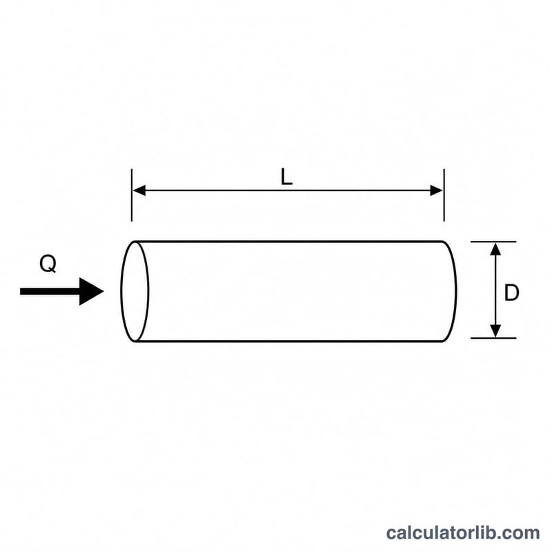
How to Use It
Enter the flow rate in liters per minute, the pipe length in meters, the internal diameter in millimeters, and the roughness coefficient. The tool converts units, computes the head loss, and also reports the average flow velocity \(v = Q / (\tfrac{\pi}{4}D^2)\).
Worked Example
For \(Q = 1000\) L/min \(= 0.01667\ \text{m}^3/\text{s}\), \(L = 100\) m, \(D = 0.1\) m, and \(C = 130\):
$$h_f = \frac{10.67 \times 100 \times 0.01667^{1.852}}{130^{1.852}\times 0.1^{4.8704}} \approx 4.90\ \text{m}$$The average velocity is \(v = 0.01667 / (0.7854 \times 0.01) \approx 2.12\ \text{m/s}\).
Hazen-Williams C Coefficients by Pipe Material
The Hazen-Williams coefficient C describes how smooth the inside of a pipe is. A higher C means less friction and less head loss. The values below are typical design ranges. They vary by source, pipe age, water quality and installation, so check the standard or manufacturer data for your project.
| Pipe material | Typical C |
|---|---|
| PVC / plastic / HDPE | 140–150 |
| New copper / brass | 130–140 |
| New cast iron | 130 |
| New welded steel | 120 |
| New ductile iron (cement-lined) | 140 |
| Concrete | 120–140 |
| Riveted steel | 110 |
| Old cast iron | 80–100 |
| Severely corroded pipe | 60–80 |
Pipes usually lose some smoothness over time through scaling, tuberculation or biofilm. For long-lived systems, designers often use a lower C than the new-pipe value. Note that the Hazen-Williams equation is an empirical formula intended for water at ordinary temperatures and turbulent flow.
Interpreting Your Head Loss and Velocity Results
Converting head to pressure. Head loss in metres of water converts to pressure with 1 m of head ≈ 9.81 kPa ≈ 1.42 psi. For example, a 4.90 m head loss corresponds to about \(4.90 \times 9.81 \approx 48.1\) kPa, or roughly 7.0 psi, lost to friction.
Head loss as a gradient. Dividing head loss by pipe length gives the hydraulic gradient. A loss of 4.9 m over 100 m is a gradient of 0.049 m/m, or 4.9 m per 100 m. The gradient lets you compare pipe options regardless of length and estimate the loss for any other length of the same pipe at the same flow.
Velocity guidelines. Water supply designs commonly target about 0.9–2.4 m/s, and 3 m/s is often cited as a maximum. Local codes and utility standards differ, so check the rules that apply to your project. Velocity is calculated as \(v = Q / A\), where \(A = \pi D^2 / 4\).
Effects of high velocity. Fast flow increases noise, can erode pipe walls and fittings (especially at bends and in softer materials), and makes pressure surges (water hammer) more severe when valves close quickly. Very low velocities, on the other hand, can let sediment settle.
Limits of the result. The calculator gives friction loss for straight pipe only. Fittings, valves, meters, entrances and exits add separate minor losses, and elevation changes add or subtract static head. Include these in a full system calculation.
Head Loss Across Diameters and Flow Rates
All values below use \(L = 100\) m and \(C = 130\), calculated with \(h_f = \dfrac{10.67 \cdot L \cdot Q^{1.852}}{C^{1.852} \cdot D^{4.8704}}\), where Q is in m³/s and D is in metres. Velocity is \(v = Q/A\). Because the length is 100 m, each head loss value is also the loss in metres per 100 m of pipe.
| Diameter (mm) | Flow (L/min) | Head loss (m) | Velocity (m/s) |
|---|---|---|---|
| 50 | 500 | 38.8 | 4.24 |
| 50 | 1000 | 143 | 8.49 |
| 50 | 1500 | 304 | 12.73 |
| 75 | 500 | 5.38 | 1.89 |
| 75 | 1000 | 19.9 | 3.77 |
| 75 | 1500 | 42.2 | 5.66 |
| 100 | 500 | 1.33 | 1.06 |
| 100 | 1000 | 4.90 | 2.12 |
| 100 | 1500 | 10.4 | 3.18 |
| 150 | 500 | 0.18 | 0.47 |
| 150 | 1000 | 0.68 | 0.94 |
| 150 | 1500 | 1.44 | 1.41 |
Reading the table. The 100 mm, 1000 L/min row matches the worked example: \(Q = 1000/60000 = 0.016667\) m³/s and \(D = 0.1\) m, so \(h_f = \dfrac{10.67 \times 100 \times 0.016667^{1.852}}{130^{1.852} \times 0.1^{4.8704}} \approx 4.90\) m, with \(v \approx 2.12\) m/s.
- Head loss grows with flow to the power 1.852, so tripling the flow raises the loss about 7.6 times.
- Head loss falls steeply with diameter, in proportion to \(D^{-4.8704}\). Doubling the diameter cuts the loss by a factor of about 29.
- The 50 mm and 75 mm rows at higher flows give velocities well above common design limits. They are shown to illustrate the trend, not as practical designs.
FAQ
When is Hazen-Williams valid? It suits water near room temperature in turbulent flow; for other fluids or wide temperature ranges use Darcy-Weisbach.
What C value should I pick? Use roughly 150 for smooth plastic, 130 for new steel, and 100 or less for old, corroded pipe.
Does diameter matter a lot? Yes, loss scales with \(D^{-4.87}\), so a small diameter increase sharply reduces friction loss.