What is the Error Function Table Calculator?
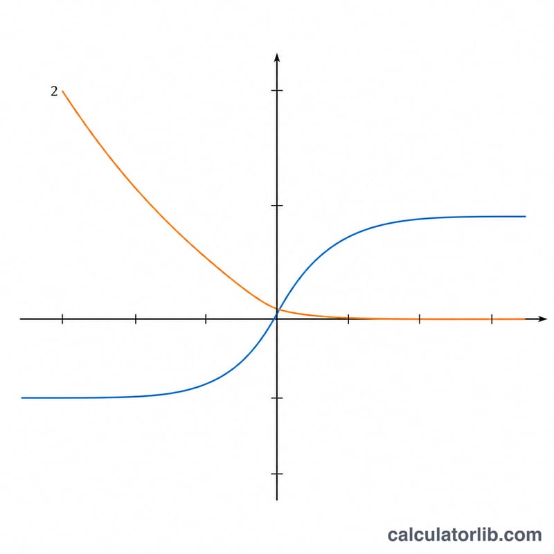
This tool builds a table of the Gauss error function erf(x) and the complementary error function erfc(x) over a sequence of x values. The error function appears throughout probability, statistics, heat conduction and diffusion problems. It is a pure mathematical (special function) tool, so it applies identically everywhere.
How to use it
Enter three numbers: the Initial value of x (the first row), the Increment added to x for each successive row, and the Number of iterations (rows). The calculator generates \(x = \text{startX} + i \times \text{stepX}\) for \(i = 0, 1, \ldots, \text{numPoints}-1\) and reports erf(x) and erfc(x) for every row. The increment may be negative (descending table) or zero (all rows identical).
The formula
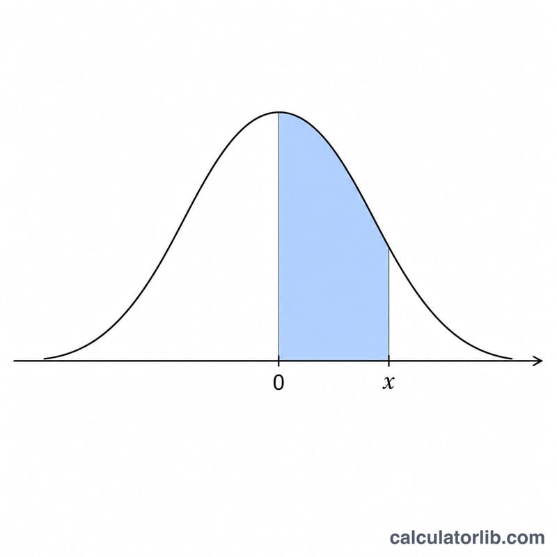
$$\operatorname{erf}(x) = \frac{2}{\sqrt{\pi}} \int_{0}^{x} e^{-t^{2}}\,dt, \qquad \operatorname{erfc}(x) = 1 - \operatorname{erf}(x)$$The values are computed with the Abramowitz & Stegun 7.1.26 rational approximation (maximum error about \(1.5 \times 10^{-7}\)), using the odd symmetry \(\operatorname{erf}(-x) = -\operatorname{erf}(x)\) for negative arguments.
Worked example
With Initial value 0, Increment 0.5 and 5 rows you get \(x = 0, 0.5, 1.0, 1.5, 2.0\). Then \(\operatorname{erf}(1.0) \approx 0.8427008\) and \(\operatorname{erfc}(1.0) \approx 0.1572992\), and indeed \(\operatorname{erf}(1.0) + \operatorname{erfc}(1.0) = 1\), confirming the identity.
Common erf(x) and erfc(x) Reference Values
The Gauss error function is \(\operatorname{erf}(x) = \frac{2}{\sqrt{\pi}}\int_0^x e^{-t^2}\,dt\), and the complementary error function is \(\operatorname{erfc}(x) = 1 - \operatorname{erf}(x)\). The table below lists widely used values, rounded to 7 decimals. You can reproduce it with start = 0, increment = 0.5 and 7 rows.
| x | erf(x) | erfc(x) |
|---|---|---|
| 0 | 0.0000000 | 1.0000000 |
| 0.5 | 0.5204999 | 0.4795001 |
| 1 | 0.8427008 | 0.1572992 |
| 1.5 | 0.9661051 | 0.0338949 |
| 2 | 0.9953223 | 0.0046777 |
| 2.5 | 0.9995930 | 0.0004070 |
| 3 | 0.9999779 | 0.0000221 |
Symmetry: erf is an odd function, so \(\operatorname{erf}(-x) = -\operatorname{erf}(x)\) and therefore \(\operatorname{erfc}(-x) = 1 + \operatorname{erf}(x) = 2 - \operatorname{erfc}(x)\). As x grows, erf(x) approaches 1 and erfc(x) approaches 0.
Interpreting erf and erfc Values
Link to the normal distribution. The standard normal cumulative distribution function is
$$\Phi(z) = \tfrac{1}{2}\left[1 + \operatorname{erf}\left(\frac{z}{\sqrt{2}}\right)\right]$$
For a normal variable X with mean μ and standard deviation σ, erf(x) is the probability of landing within x·σ·√2 of the mean:
$$P\left(|X-\mu| \le x\,\sigma\sqrt{2}\right) = \operatorname{erf}(x)$$
Examples:
- \(\operatorname{erf}(1/\sqrt{2}) \approx 0.6827\): about 68.27% of values lie within ±1σ.
- \(\operatorname{erf}(2/\sqrt{2}) \approx 0.9545\): about 95.45% of values lie within ±2σ.
- \(\operatorname{erf}(3/\sqrt{2}) \approx 0.9973\): about 99.73% of values lie within ±3σ.
erfc as a tail probability. erfc(x) is the probability of falling outside that central band, i.e. both tails combined. With Q(z) = 1 − Φ(z) as the upper-tail probability, \(\operatorname{erfc}(x) = 2\,Q(x\sqrt{2})\). For example, erfc(1/√2) ≈ 0.3173, the two-sided probability beyond ±1σ.
Accuracy note. Many fast implementations use a rational approximation (for example the Abramowitz and Stegun formula) with a maximum absolute error of about 1.5×10⁻⁷. That is plenty for erf(x) itself, but erfc(x) = 1 − erf(x) becomes very small for large x (erfc(3) ≈ 2.2×10⁻⁵, erfc(5) ≈ 1.5×10⁻¹²). An absolute error of 10⁻⁷ therefore removes most or all of the significant digits in far-tail values. Treat very small erfc entries at large x as approximate, and use a dedicated high-precision erfc routine if you need accurate extreme-tail probabilities.
FAQ
What range can erf take? \(\operatorname{erf}(x)\) lies in \((-1, 1)\); \(\operatorname{erf}(0) = 0\), \(\operatorname{erf}(+\infty) = 1\), \(\operatorname{erf}(-\infty) = -1\).
What about erfc? \(\operatorname{erfc}(x)\) lies in \((0, 2)\): \(\operatorname{erfc}(0) = 1\), \(\operatorname{erfc}(+\infty) = 0\), \(\operatorname{erfc}(-\infty) = 2\).
How many rows can I generate? The number of rows must be a positive integer; the table is capped at 2000 rows to keep output manageable.