What this calculator does
A grid-tied (on-grid) solar system has no battery: it feeds the house first and exports any surplus to the utility. Sizing it therefore comes down to matching yearly generation to yearly consumption. This calculator turns your monthly electricity bill, your local peak sun hours and the wattage of the module you plan to buy into a panel count, a DC array size in kilowatts, a suggested inverter rating, an annual yield estimate and a rough roof-area requirement. The method is universal — it uses only physics and equipment ratings, not any country specific incentive or tariff rule.
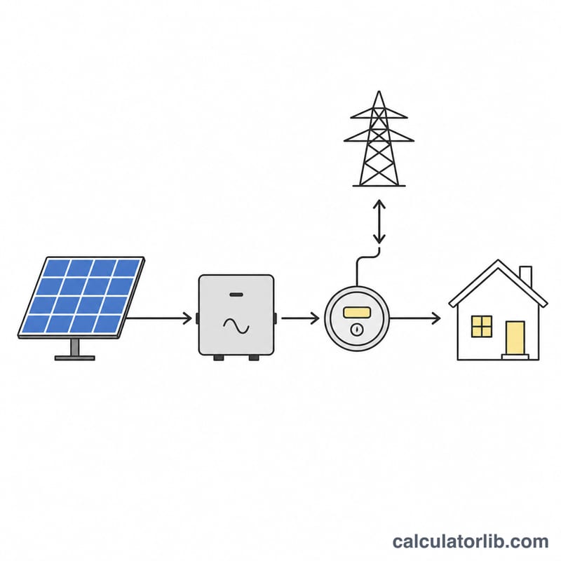
How to use it
Enter your average monthly consumption in kWh (read it off a bill, or average twelve months). Enter peak sun hours for your site — the number of hours per day of 1000 W/m² equivalent irradiance, typically 3.0 to 4.5 in northern Europe, 4.5 to 5.5 in most of the US and 4.5 to 5.0 across Southeast Asia. Choose your panel rating (400-600 W for modern modules) and a system efficiency between 75% and 85%. Set the bill offset below 100% if you only want to cover part of your usage.
The formula
With \(E_{\text{daily}}\) = daily consumption in kWh, \(O\) = target offset, \(H\) = peak sun hours, \(\eta\) = system efficiency and \(P_{\text{panel}}\) = panel watts, the array size and panel count are
$$P_{\text{array}} = \frac{E_{\text{daily}} \times O}{H \times \eta}, \qquad N = \left\lceil \frac{1000 \times P_{\text{array}}}{P_{\text{panel}}} \right\rceil$$Daily use comes from the monthly figure via \(E_{\text{daily}} = E_{\text{month}} / 30.44\), the average days per month.
Worked example
A home uses 900 kWh per month at a site with 5 peak sun hours, using 550 W panels at 80% system efficiency and a 100% offset:
$$E_{\text{daily}} = \frac{900}{30.44} = 29.57\,\text{kWh}$$$$P_{\text{array}} = \frac{29.57}{5 \times 0.80} = 7.39\,\text{kW}$$$$N = \left\lceil \frac{7392}{550} \right\rceil = \left\lceil 13.44 \right\rceil = 14\ \text{panels}$$Fourteen panels give 7.7 kW installed and roughly \(7.7 \times 5 \times 0.8 \times 365 = 11242\) kWh per year.

Peak Sun Hours by Region
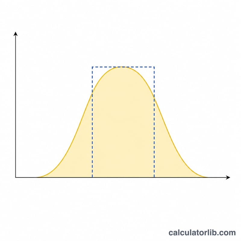
"Peak sun hours" (PSH) is the number of hours per day that solar irradiance would have to sit at exactly 1000 W/m² to deliver the same daily energy as the real, varying sun. It is numerically identical to daily irradiation expressed in kWh/m²/day, which is why a site with 4.5 kWh/m²/day is said to have 4.5 peak sun hours. This is the value the sizing formula uses as \(H\).
| Region / example location | Typical annual-average PSH (kWh/m²/day) | Note |
|---|---|---|
| UK, Ireland, northern Germany, southern Scandinavia | 2.5 – 3.0 | Strong summer/winter swing; winter can fall below 1 |
| Central Europe (France, S. Germany, Poland, N. Italy) | 3.0 – 3.5 | Moderate seasonality |
| Southern Europe (Spain, S. Italy, Greece, Portugal) | 4.5 – 5.0 | High summer yield, mild winters |
| US Northeast / Upper Midwest | 4.0 – 4.5 | Snow cover can interrupt winter output |
| US Southwest (Arizona, Nevada, New Mexico) | 5.5 – 6.5 | Among the highest resource areas worldwide |
| India (most of the country) | 5.0 – 5.5 | Monsoon months reduce mid-year output |
| Southeast Asia (Vietnam, Thailand, Indonesia, Philippines) | 4.0 – 5.0 | High cloud cover offsets low latitude |
| Australia (populated south and east) | 4.5 – 5.5 | Higher again in the arid interior and north-west |
These bands are rounded, representative annual averages drawn from public irradiance databases — chiefly the US NREL National Solar Radiation Database (NSRDB) and the European Commission's PVGIS, both of which report long-term satellite-derived irradiation for a given latitude and longitude. They are illustrative regional figures, not a substitute for a lookup at your own coordinates.
Your site-specific value can differ from the regional band by 10–25% because PSH on the array plane depends on more than location:
- Tilt — a tilt near the site latitude maximises annual energy; a flat (0°) array in a high-latitude country loses noticeably more than in the tropics.
- Azimuth — true south in the northern hemisphere, true north in the southern hemisphere is optimal; east or west facing typically costs roughly 10–20% of annual yield.
- Shading and horizon — trees, chimneys, parapets and neighbouring buildings reduce effective PSH, and partial shading of one module can drag down a whole string unless optimisers or microinverters are used.
- Local climate — coastal fog, monsoon seasons, dust and persistent haze all lower the long-run average.
If you have a PVGIS or NSRDB figure for your exact roof plane, use that number instead of the regional band above.
Typical Values for System Efficiency, DC/AC Ratio and Panel Wattage
System efficiency (performance ratio), \(\eta\): 0.75 – 0.85
The derate factor converts nameplate DC capacity into energy actually delivered to the grid. It is the product of several independent loss terms, so the losses multiply rather than simply add:
| Loss mechanism | Typical loss | What drives it |
|---|---|---|
| Soiling (dust, pollen, bird droppings) | 2 – 5% | Dry/dusty climates and low tilt angles sit at the high end |
| Cell temperature above 25 °C | 5 – 12% | Module temperature coefficient (roughly −0.3 to −0.4%/°C); hot, still climates and tight roof mounting are worst |
| Wiring, connectors and module mismatch | 2 – 3% | DC/AC cable runs, string mismatch, tolerance spread |
| Inverter conversion | 2 – 4% | Modern string inverters peak near 97–98% efficiency |
| Shading, snow, availability, clipping | 0 – 5%+ | Highly site-specific; excluded from the "clean site" figure |
A well-designed, unshaded rooftop system commonly lands at \(\eta \approx 0.80\) (80%), which is the sensible default. Use 0.85 only for a cool, clean, well-ventilated array, and 0.75 or below for hot, dusty or partially shaded sites. A worked check for the four core losses:
$$\eta = 0.97 \times 0.92 \times 0.975 \times 0.97 = 0.844$$DC/AC (inverter loading) ratio: 1.1 – 1.3, with 1.2 the common default
The inverter is deliberately sized smaller than the DC array, because the array almost never reaches its STC nameplate output in the field. The ratio is
$$\text{DC/AC ratio} = \frac{\text{Array DC rating (kW)}}{\text{Inverter AC rating (kW)}}$$So an 8.25 kW array at a 1.2 ratio calls for an inverter of about \(8.25 \div 1.2 = 6.9\) kW AC. Higher ratios (1.25–1.3) suit diffuse, cloudy climates or east–west arrays where peaks are rare; lower ratios (1.1–1.15) suit very sunny, cool, south-facing arrays where clipping would otherwise waste energy. Note that grid-connection rules in some countries cap the exportable AC rating or the permitted DC:AC ratio (for example, many Australian distribution networks and several European feed-in schemes set explicit limits), so confirm the local requirement with your utility or installer before fixing the inverter size.
Module rating and area: 400 – 600 W at roughly 2.0 – 2.3 m²
Mainstream residential and commercial modules sold today are rated around 400–600 W under standard test conditions, with a physical area of roughly 2.0–2.3 m² each. That corresponds to about 200–220 W/m² of module surface, equivalent to a module conversion efficiency of roughly 20–22%. A practical planning rule:
$$\text{Roof area (m}^2) \approx N \times 2.0 \text{ to } 2.3$$Add 20–40% on top of that for row spacing, walkways, setbacks and fire-access paths — many jurisdictions mandate clear perimeter and ridge access on residential roofs.
Annual degradation: 0.4 – 0.7% per year
Modules lose a small amount of output each year. Typical 25-year performance warranties from major manufacturers guarantee something on the order of 80–87% of initial rated output at year 25, which implies a linear degradation allowance of roughly 0.4–0.7%/yr (often with a larger first-year step of about 1–2%). To estimate output in a later year:
$$E_{\text{year }n} = E_1 \times (1 - d)^{\,n-1}$$With \(E_1 = 7358\) kWh and \(d = 0.005\), year 25 output is \(7358 \times (1-0.005)^{24} = 7358 \times 0.8866 \approx 6524\) kWh. Sizing calculators — including this one — normally report year-one output, so treat the figure as the starting point of a slowly declining curve.
Sizing Across Different Homes and Climates
The table below applies the article's formulas to six combinations of household consumption, solar resource and module rating, all at a system efficiency of 80% (\(\eta = 0.80\)) and a target offset of 100%. Each row is computed as:
$$E_d = \frac{\text{Monthly kWh}}{30.44}, \qquad N = \left\lceil \frac{1000 \cdot E_d}{H \cdot \eta \cdot W_p} \right\rceil, \qquad P_{dc} = \frac{N \cdot W_p}{1000}$$$$P_{ac} = \frac{P_{dc} }{1.2}, \qquad E_{\text{year}} = P_{dc} \cdot H \cdot \eta \cdot 365$$| Monthly use (kWh) | Peak sun hours | Panel (W) | Panels \(N\) | Array kW (DC) | Inverter kW (AC, 1.2 ratio) | Est. annual kWh | Approx. module area |
|---|---|---|---|---|---|---|---|
| 300 | 3.0 | 400 | 11 | 4.40 | 3.7 | 3,854 | 22 m² |
| 600 | 4.5 | 400 | 14 | 5.60 | 4.7 | 7,358 | 28 m² |
| 900 | 4.5 | 550 | 15 | 8.25 | 6.9 | 10,841 | 34.5 m² |
| 900 | 5.5 | 550 | 13 | 7.15 | 6.0 | 11,483 | 29.9 m² |
| 1500 | 5.5 | 550 | 21 | 11.55 | 9.6 | 18,549 | 48.3 m² |
| 1500 | 3.0 | 400 | 52 | 20.80 | 17.3 | 18,221 | 104 m² |
Module area assumes 2.0 m² per 400 W panel and 2.3 m² per 550 W panel; usable roof area must be larger to allow for spacing, setbacks and access paths.
Row 2 worked in full
A 600 kWh/month home at 4.5 peak sun hours with 400 W modules:
$$E_d = \frac{600}{30.44} \times \frac{100}{100} = 19.71 \text{ kWh/day}$$$$N = \left\lceil \frac{1000 \times 19.71}{4.5 \times 0.80 \times 400} \right\rceil = \left\lceil \frac{19{,}710}{1440} \right\rceil = \lceil 13.69 \rceil = 14 \text{ panels}$$$$P_{dc} = \frac{14 \times 400}{1000} = 5.60 \text{ kW}, \qquad P_{ac} = \frac{5.60}{1.2} = 4.67 \text{ kW}$$$$E_{\text{year}} = 5.60 \times 4.5 \times 0.80 \times 365 = 7{,}358 \text{ kWh}$$Rounding \(N\) up means the system slightly overshoots the 7,200 kWh annual load — 7,358 kWh, an offset of about 102%.
What the rows show
- Solar resource dominates. The same 1500 kWh/month load needs 11.55 kW at 5.5 sun hours but 20.8 kW at 3.0 — an 80% larger array for essentially the same annual energy.
- Panel wattage changes the count, not the kW. Going from 400 W to 550 W modules cuts the panel count and the number of mounting points, while the array kW stays roughly the same for a given load. It mainly buys back roof space.
- Ceiling rounding matters most on small systems. At 11 panels, one extra module is a ~9% oversize; at 52 panels it is under 2%.
- Inverter sizing is a design choice, not a fixed output. The 1.2 ratio used here is a common default — check what your grid operator permits before ordering.
Two caveats before treating any row as a quote. First, a 100% annual offset does not mean self-sufficiency: a grid-tied system without storage still draws from the grid at night and exports at midday, and how that is settled — net metering, net billing or a flat export tariff — is set by national or state rules that vary widely, so check your local scheme. Second, these are year-one energy estimates at a generic 80% derate; a site-specific quote should use measured shading, your actual roof tilt and azimuth, and a PVGIS or NSRDB irradiance lookup for your coordinates.
FAQ
Why is the inverter smaller than the array? Panels rarely hit their nameplate rating, so a DC/AC ratio near 1.2 is standard — it keeps the inverter working in its efficient range with almost no clipping loss.
What efficiency should I use? 80% is a safe default. Drop to 72-75% for hot climates, long cable runs, dust or partial shading; 85% is optimistic and only realistic for cool, clean, ideally oriented roofs.
Does a bigger system always pay? Not on-grid. If your utility pays little for exported energy, sizing to about 80-90% of consumption usually returns more than a system that overproduces every summer.