What is the sigmoid function?
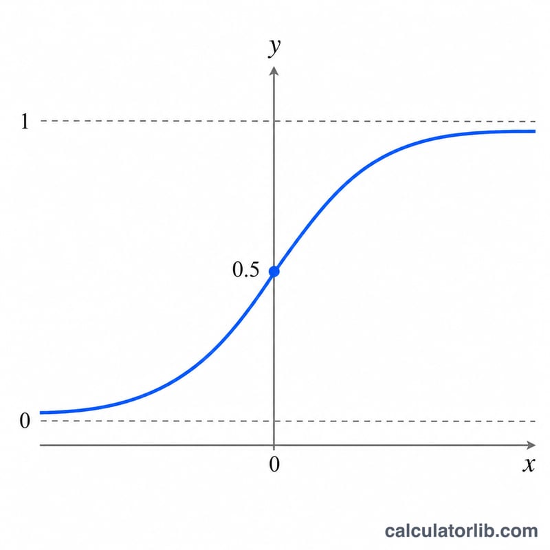
The sigmoid, or logistic, function squashes any real number into the open interval (0, 1) with a smooth S-shaped curve. Defined as \(\sigma(x) = \frac{1}{1 + e^{-\text{a}\,x}}\), it is one of the most widely used activation functions in neural networks and a staple of logistic regression, probability modeling and growth curves. The gain parameter \(\text{a}\) controls how steep the transition is: with \(\text{a} = 1\) you get the classic textbook sigmoid, while larger \(\text{a}\) values compress the transition toward a step function.
How to use this calculator
Enter the gain \(\text{a}\), then the range over which you want to evaluate the function: x minimum, x maximum and the x step (increment). The tool builds a table of \(\sigma(x)\), its first derivative \(\sigma^{\prime}(x)\) and second derivative \(\sigma^{\prime\prime}(x)\) at each step, and reports the single-point values at the optional x you supply. Make sure the step is greater than zero and that x maximum is at least x minimum, otherwise no rows are produced.
The formulas explained
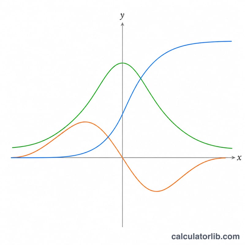
The derivatives have especially clean forms when written in terms of \(\sigma\) itself. Differentiating gives $$\sigma^{\prime}(x) = \text{a}\,\sigma(x)\bigl(1 - \sigma(x)\bigr)$$ which is always positive (the curve is monotonically increasing) and reaches its maximum value of \(\frac{\text{a}}{4}\) at the inflection point \(x = 0\). The second derivative, $$\sigma^{\prime\prime}(x) = \text{a}^{2}\,\sigma(x)\bigl(1 - \sigma(x)\bigr)\bigl(1 - 2\,\sigma(x)\bigr)$$ changes sign at \(x = 0\) where \(\sigma = 0.5\), confirming the inflection point.
Worked example
Take \(\text{a} = 1\) and \(x = 2\). Then \(e^{-2} = 0.135335\), so $$\sigma(2) = \frac{1}{1.135335} = 0.880797$$ The first derivative is $$0.880797 \times (1 - 0.880797) = 0.104994$$ The second derivative is $$0.104994 \times (1 - 2 \times 0.880797) = 0.104994 \times (-0.761594) = -0.079963$$ At \(x = 0\) the values are \(\sigma = 0.5\), \(\sigma^{\prime} = 0.25\) and \(\sigma^{\prime\prime} = 0\).
FAQ
What does the gain a do? It scales the input. A larger \(\text{a}\) makes the curve rise faster around \(x = 0\); as \(\text{a}\) grows the sigmoid approaches a hard step, while \(\text{a} = 0\) gives a flat line at 0.5.
Where is the steepest point? Always at \(x = 0\), where the slope equals \(\frac{\text{a}}{4}\) and the second derivative is zero.
Why is the output never exactly 0 or 1? The exponential never reaches zero for finite x, so \(\sigma\) stays strictly inside (0, 1). For extremely large \(|\text{a}\,x|\) the value rounds to 0 or 1 numerically, which this calculator handles safely.


