What this calculator does
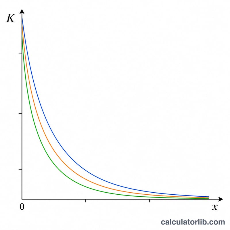
This tool tabulates and plots the modified Bessel function of the second kind, written \(K_{\nu}(x)\). Given a fixed real order \(\nu\) and a sweep of x-values, it returns a two-column table of x versus \(K_{\nu}(x)\) together with a line graph showing how the function decays. It is pure mathematics and applies universally with no regional assumptions.
Background
The modified Bessel functions are the two independent solutions of the modified Bessel equation \(x^2 y'' + x y' - (x^2 + \nu^2)y = 0\). The first kind \(I_{\nu}(x)\) grows; the second kind \(K_{\nu}(x)\) decays exponentially. Note that \(K_{\nu}(x) = K_{-\nu}(x)\), so the sign of the order does not matter — the calculator uses \(|\nu|\) internally.
How to use it
Enter the Order \(\nu\) (any real number), the Initial value of x, the Increment added to x for each row, and the Number of repetitions (the count of x sample points / table rows). Row i uses \(x = \text{startX} + i\cdot\text{stepX}\). Because \(K_{\nu}(x)\) is only defined for \(x > 0\) and diverges to \(+\infty\) as \(x\to 0^{+}\), a row at \(x = 0\) (or negative x) is reported as Infinity.
The formula explained
The calculator evaluates the integral representation $$K_{\nu}(x) = \int_{0}^{\infty} e^{-x \cosh t}\,\cosh\!\left(\nu\, t\right)\,dt$$ using composite Simpson quadrature. The upper limit is truncated where the integrand becomes negligible (when \(x\cdot\cosh t\) exceeds about 45). This form has no singularity at integer orders, so \(K_0\), \(K_1\), … are handled directly without the 0/0 problem of the closed form involving \(I_{\nu}\).
Worked example
With \(\nu = 0\), \(\text{startX} = 0.1\), \(\text{stepX} = 0.1\), iterations = 3 the table is: $$x = 0.1 \rightarrow 2.427069, \quad x = 0.2 \rightarrow 1.752704, \quad x = 0.3 \rightarrow 1.372460.$$ These match standard tabulated values of \(K_0\).
FAQ
Why is the first value sometimes \(\infty\)? Because \(K_{\nu}(0)\) diverges; choose a small positive startX such as 0.1.
Does a negative order work? Yes — \(K_{\nu}(x) = K_{-\nu}(x)\), so the result for \(-\nu\) equals the result for \(\nu\).
Why do large-x values become 0? \(K_{\nu}(x)\) decays like \(\sqrt{\pi/2x}\cdot e^{-x}\), so it underflows to 0 for large x, which is correct.


