Inverse Incomplete Beta Function Calculator

Enter Calculation

Results

Inverse value x

0.5358411166

upper limit such that the chosen beta function equals y

Complete beta B(a,b)	0.3333333333
Regularized target p = I_x(a,b)	0.9

What this calculator does

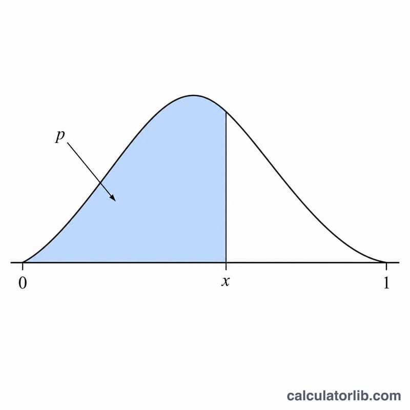
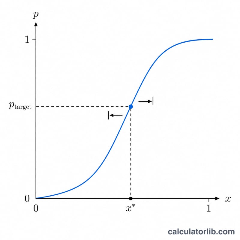
The inverse incomplete beta function calculator finds the upper integration limit x for which a chosen beta function reaches a target value y. You can invert either the non-normalized incomplete beta function $B_x(a,b)$ or the regularized (normalized) version $I_x(a,b)$. Because $I_x(a,b)$ increases monotonically from 0 to 1, this inversion is exactly the quantile (percent-point) operation behind the beta distribution and the critical values of the Student t, Fisher F and binomial distributions.

Beta density curve with shaded left area p ending at point x — The regularized incomplete beta I_x(a,b) is the shaded area p; the inverse finds the x that gives a target p.

How to use it

Pick the Function you want to invert. Enter the target y, and the two positive shape parameters a and b. For the regularized mode, y must lie between 0 and 1. For the non-normalized mode, y must lie between 0 and the complete beta value $B(a,b)$, which the result panel reports for you. Both a and b must be strictly greater than 0.

The formula and the algorithm

The complete beta is computed as $$B(a,b)=\exp\bigl(\ln\Gamma(a)+\ln\Gamma(b)-\ln\Gamma(a+b)\bigr).$$ The target is converted to a regularized probability p ($p=y$ for $I_x$, $p=y/B(a,b)$ for $B_x$). The forward $I_x(a,b)$ is evaluated with a continued fraction (modified Lentz iteration) using the standard symmetric-argument trick for stability, and the equation $I_x(a,b)=p$ is solved by bisection on $[0,1]$, which is guaranteed to converge.

Monotonic I_x curve with dashed lines mapping a target p back to the solution x — Because I_x(a,b) increases monotonically in x, the inverse is found by root-finding for the x where the curve hits target p.

Worked example

Take the regularized mode with y = 0.3, a = 1, b = 3. With a = 1 the identity $I_x(1,b)=1-(1-x)^b$ applies, so $$1-(1-x)^3=0.3$$ gives $(1-x)^3=0.7$, hence $1-x = 0.887904$ and $x \approx 0.1120959$. In non-normalized mode with the same y,a,b: $B(1,3)=1/3$, so $p=0.3/(1/3)=0.9$, giving $(1-x)^3=0.1$ and $x \approx 0.5358407$.

FAQ

What is the difference between $B_x$ and $I_x$? $I_x$ is $B_x$ divided by the complete beta $B(a,b)$, so $I_x$ always ranges 0 to 1 while $B_x$ ranges 0 to $B(a,b)$.

Why must a and b be positive? The defining integral converges only for $a>0$ and $b>0$; otherwise the Gamma function and the integral are undefined.

How accurate is the result? The root finder converges to about double precision (~15 significant digits), which is more than enough for statistical quantile work.

Related calculators

Incomplete Beta Function Calculator

Compute the lower incomplete beta function B_x(a,b) by numerically integrating t^(a-1)(1-t)^(b-1) with Gauss-Legendre quadrature. Set x=1 for the complete beta function.

Beta Function B(a,b) Calculator

Compute the Euler Beta function B(a,b) for any two real arguments using the gamma-ratio form and numerically stable log-gamma. Symmetric, fast, accurate.

Inverse Function Calculator

Find the inverse f⁻¹(x) of a linear or rational function f(x)=(ax+b)/(cx+d). Get the inverse formula and evaluate it at any x value instantly.

Incomplete Beta Function & Regularized Incomplete Beta Function Table Calculator

Build a table of the lower incomplete beta function Bx(a,b) and the regularized incomplete beta Ix(a,b) over a range of x for given shape parameters a and b.

Inverse Trigonometric Function Calculator

Compute arcsin, arccos, arctan, arccot, arcsec or arccsc of a value. Get the principal-value angle in degrees or radians, plus domain and range.

Incomplete Gamma Function Calculator

Compute the lower incomplete gamma function gamma(a,x) and upper incomplete gamma function Gamma(a,x) for any a > 0 and x ≥ 0, plus the complete gamma Gamma(a).