What this calculator does
This tool computes and plots the one-dimensional quantum harmonic oscillator (QHO) wavefunction \(\psi_n(x)\) for a chosen quantum number \(n\) over a range of positions \(x\). The QHO is one of the most important exactly solvable models in quantum mechanics, describing vibrating molecules, phonons in solids, and modes of the electromagnetic field. The wavefunctions are the eigenstates of the Hamiltonian with energies \(E_n = \hbar\omega(n + \tfrac{1}{2})\).
Unit convention
To keep the result purely numerical, positions are measured in dimensionless oscillator-length units, which is equivalent to setting the parameter \(\alpha = \sqrt{m\omega/\hbar} = 1\). With this choice no mass, angular frequency or \(\hbar\) values are needed: you only supply \(n\) and the \(x\) sampling parameters. Energies come out in units of \(\hbar\omega\), so \(E_n\) simply equals \(n + \tfrac{1}{2}\).
The formula
The normalized eigenfunction is $$\psi_n(x) = N_n\, H_n(x)\, e^{-x^{2}/2},$$ where the normalization constant \(N_n = \sqrt{1 / (2^{n}\, n!\, \sqrt{\pi})}\) and \(H_n\) is the physicists' Hermite polynomial. Hermite polynomials are built from the stable recurrence \(H_0 = 1\), \(H_1 = 2x\), and \(H_{k+1} = 2x\,H_k - 2k\,H_{k-1}\). The normalization is computed in the log domain to avoid overflow at large \(n\).
How to use it
Enter the quantum number \(n\) (0, 1, 2, ...), the initial position \(x\), the step size, and the number of points to sample. The calculator evaluates \(x_i = \text{startX} + i\cdot\text{stepX}\) for each \(i\) and returns \(\psi\) at each point plus a graph of \(\psi(x)\) versus \(x\). The defaults (start -4, step 0.1, 81 points) sweep \(x\) from -4 to +4.
Worked example
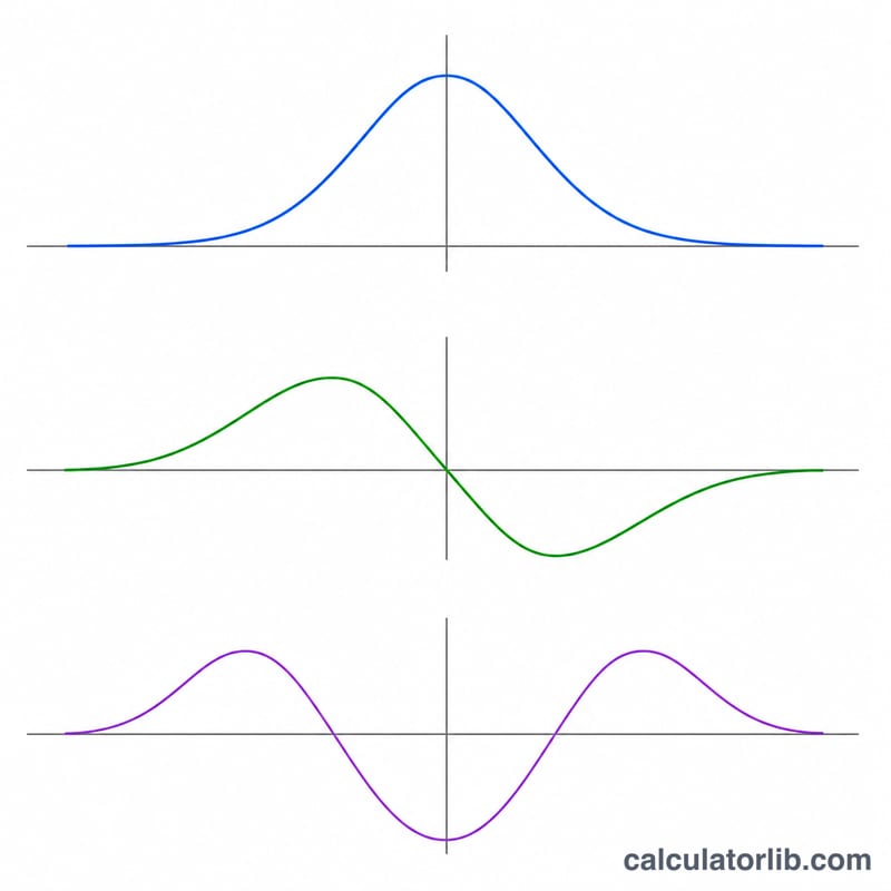
For \(n = 1\) at \(x = 1.0\): \(N_1 = \sqrt{1/(2\sqrt{\pi})} = 0.5311259\), \(H_1(1) = 2.0\), and \(e^{-0.5} = 0.6065307\). Therefore $$\psi_1(1.0) = 0.5311259 \times 2.0 \times 0.6065307 = 0.6442715.$$ The \(n = 1\) state has a node at \(x = 0\), where \(\psi_1(0) = 0\).
FAQ
Why does \(\psi\) go negative? Wavefunctions are real here and oscillate in sign; the physically observable probability density is \(|\psi|^2\), which is always non-negative.
How many nodes does \(\psi_n\) have? Exactly \(n\) nodes (zero crossings) inside the well, a hallmark of the \(n\)-th excited state.
Is \(\psi\) normalized? Yes, in continuous \(x\) the integral of \(\psi_n^2\, dx\) equals 1. A finite sampled grid only approximates that integral.