
What is the logistic distribution?
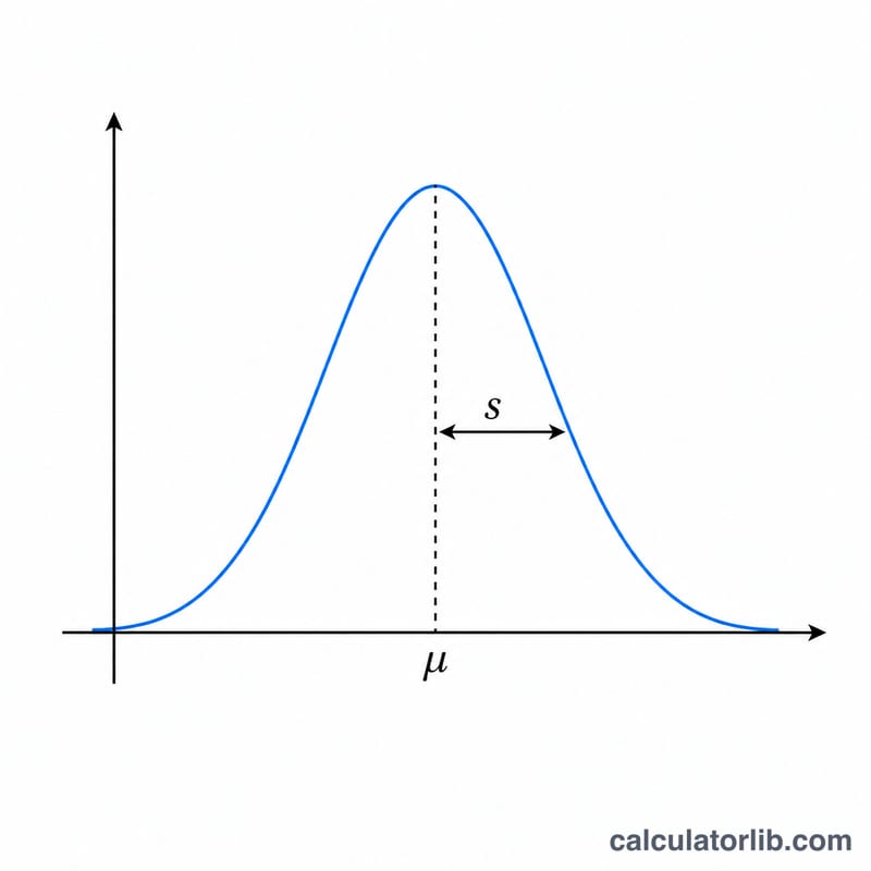
The logistic distribution is a continuous probability distribution shaped like the normal distribution but with heavier tails. It is defined by a location parameter (its mean) \(\mu\) and a positive scale parameter \(s\). Its cumulative distribution function is the well-known logistic sigmoid, which is why the distribution appears throughout statistics, machine learning (logistic regression), and growth modeling. This calculator is pure mathematics and applies identically everywhere.
How to use it
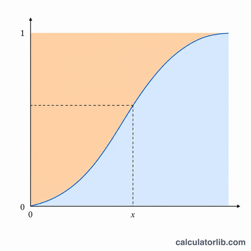
Enter the value \(x\) at which you want to evaluate the distribution, the location parameter \(\mu\) (the mean, which is also the center of symmetry), and the scale parameter \(s\), which must be strictly positive. The calculator returns three numbers: the probability density \(f(x)\), the lower cumulative probability \(P(X \le x)\), and the upper cumulative probability \(P(X > x)\). The two cumulative probabilities always sum to 1.
The formulas explained
First compute the standardized value \(z = (x - \mu) / s\). The lower CDF is $$F(x) = \frac{1}{1 + e^{-z}}.$$ The density is $$f(x) = \frac{e^{-z}}{s\left(1 + e^{-z}\right)^{2}},$$ which equals \(F(x)(1 - F(x))/s\). The upper (survival) probability is $$S(x) = 1 - F(x) = \frac{e^{-z}}{1 + e^{-z}}.$$ To stay numerically stable for large \(|z|\), the sigmoid is computed differently for positive and negative \(z\) so \(\exp()\) never overflows.
Worked example
Suppose \(x = 2\), \(\mu = 1\), \(s = 2\). Then \(z = (2 - 1)/2 = 0.5\) and \(e^{-0.5} = 0.606531\). The lower CDF is $$F = \frac{1}{1 + 0.606531} = 0.622459.$$ The upper CDF is \(1 - 0.622459 = 0.377541\). The density is $$f = \frac{0.622459 \times 0.377541}{2} = 0.117493.$$
FAQ
What does the scale parameter do? A larger \(s\) spreads the distribution out and lowers the peak; a smaller \(s\) makes it sharper. The peak density at \(x = \mu\) equals \(1/(4s)\).
Can mu or x be negative? Yes. Both \(x\) and \(\mu\) can be any real number. Only \(s\) must be positive.
How does it relate to the standard logistic? With \(\mu = 0\) and \(s = 1\) you get the standard logistic distribution; at \(x = 0\) the density is 0.25 and both cumulative probabilities are 0.5.