What this calculator does
The Mean and Standard Deviation Calculator takes a list of numbers and returns the mean (average), the variance, and the standard deviation. The mean describes the center of your data, while the standard deviation measures how spread out the values are around that center. A small standard deviation means values cluster tightly near the mean; a large one means they are widely dispersed.
How to use it
Type or paste your numbers into the input box, separated by commas or spaces. Choose Sample if your data is a subset drawn from a larger group, or Population if it represents the entire group. The calculator then reports the mean, variance, standard deviation, count, and sum.
The formulas explained
First compute the mean \(\bar{x}\), where \(n\) is the count of values and \(x_i\) is each value:
$$\bar{x} = \frac{1}{n}\sum_{i=1}^{n} x_i$$Then measure each value deviation from the mean, square it, and average the squares. The sample version divides by \(n-1\); the population version divides by \(n\):
$$s = \sqrt{\frac{1}{n-1}\sum_{i=1}^{n}(x_i - \bar{x})^2} \qquad \sigma = \sqrt{\frac{1}{n}\sum_{i=1}^{n}(x_i - \mu)^2}$$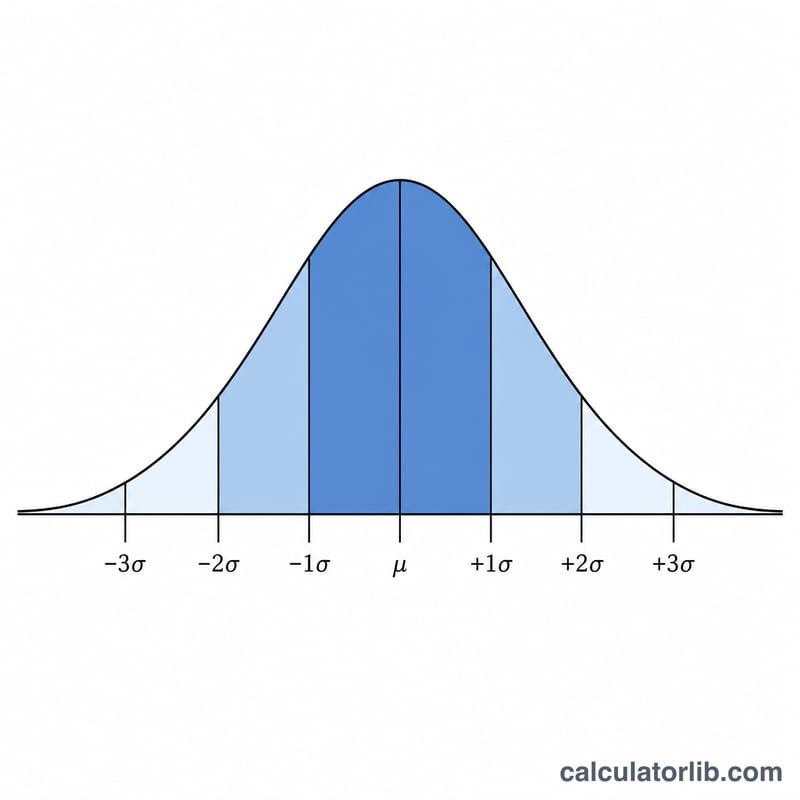
Worked example
Take the data set 2, 4, 4, 4, 5, 5, 7, 9. There are \(n = 8\) values that add to 40, so the mean is:
$$\bar{x} = \frac{2+4+4+4+5+5+7+9}{8} = 5$$The squared deviations from 5 sum to 32. Using the population formula:
$$\sigma = \sqrt{\frac{32}{8}} = \sqrt{4} = 2$$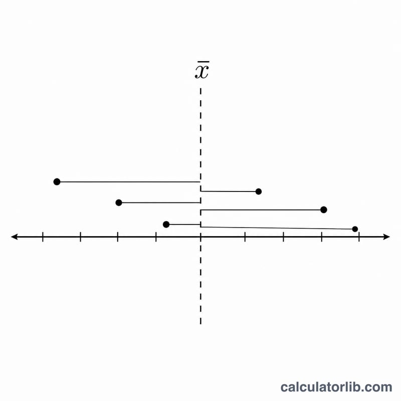
More Worked Examples
These examples use the same procedure every time: find the mean \(\bar{x}\), subtract it from each value to get the deviations, square those deviations, add them up, divide by \(n-1\) for a sample or by \(n\) for a population, and finally take the square root. The only difference between the two versions of the standard deviation is what you divide by.
Example 1 — sample vs. population on the same data
Data set (8 values): 2, 4, 4, 4, 5, 5, 7, 9.
Step 1 — mean:
$$\bar{x} = \frac{2+4+4+4+5+5+7+9}{8} = \frac{40}{8} = 5$$Step 2 — squared deviations:
| \(x_i\) | \(x_i - \bar{x}\) | \((x_i - \bar{x})^2\) |
|---|---|---|
| 2 | -3 | 9 |
| 4 | -1 | 1 |
| 4 | -1 | 1 |
| 4 | -1 | 1 |
| 5 | 0 | 0 |
| 5 | 0 | 0 |
| 7 | 2 | 4 |
| 9 | 4 | 16 |
Step 3 — sum of squares:
$$\sum_{i=1}^{n}(x_i - \bar{x})^2 = 9+1+1+1+0+0+4+16 = 32$$Step 4 — variance and standard deviation. With \(n = 8\):
Sample (divide by \(n-1 = 7\)):
$$s^2 = \frac{32}{7} \approx 4.5714 \qquad s = \sqrt{4.5714} \approx 2.1381$$Population (divide by \(n = 8\)):
$$\sigma^2 = \frac{32}{8} = 4 \qquad \sigma = \sqrt{4} = 2$$So the same data gives a sample standard deviation of 2.1381 and a population standard deviation of 2. The sample value is slightly larger because dividing by the smaller number \(n-1\) inflates the result — this is the standard correction used when the data is only a sample drawn from a larger group.
Example 2 — decimal and negative values
Data set (5 values): -2, -1, 0, 3, 5.
Mean:
$$\bar{x} = \frac{-2 + (-1) + 0 + 3 + 5}{5} = \frac{5}{5} = 1$$Squared deviations:
| \(x_i\) | \(x_i - \bar{x}\) | \((x_i - \bar{x})^2\) |
|---|---|---|
| -2 | -3 | 9 |
| -1 | -2 | 4 |
| 0 | -1 | 1 |
| 3 | 2 | 4 |
| 5 | 4 | 16 |
Sum of squares:
$$\sum_{i=1}^{n}(x_i - \bar{x})^2 = 9+4+1+4+16 = 34$$Variance and standard deviation (with \(n = 5\)):
$$s^2 = \frac{34}{4} = 8.5 \qquad s = \sqrt{8.5} \approx 2.9155$$$$\sigma^2 = \frac{34}{5} = 6.8 \qquad \sigma = \sqrt{6.8} \approx 2.6077$$Negative values are handled exactly like positive ones — squaring the deviations removes the sign, so a value below the mean contributes just as much spread as one the same distance above it.
Example 3 — evenly spaced values
Data set (5 values): 10, 20, 30, 40, 50.
Mean:
$$\bar{x} = \frac{10+20+30+40+50}{5} = \frac{150}{5} = 30$$Squared deviations: the deviations are -20, -10, 0, 10, 20, so the squares are 400, 100, 0, 100, 400.
$$\sum_{i=1}^{n}(x_i - \bar{x})^2 = 400+100+0+100+400 = 1000$$Variance and standard deviation (with \(n = 5\)):
$$s^2 = \frac{1000}{4} = 250 \qquad s = \sqrt{250} \approx 15.8114$$$$\sigma^2 = \frac{1000}{5} = 200 \qquad \sigma = \sqrt{200} \approx 14.1421$$Even though the values are perfectly evenly spaced, the standard deviation is not the spacing itself (10) — it is a root-mean-square measure of distance from the mean, which here works out to about 14.14 for the whole population.
Interpreting Your Result
The standard deviation tells you the typical distance between a data value and the mean, expressed in the same units as your data. A small standard deviation means the values cluster tightly around the mean; a large one means they are widely scattered. On its own the number is most useful when compared with the mean and with the spread of other data sets measured the same way.
The empirical (68–95–99.7) rule
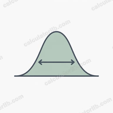
When a data set is approximately normally distributed (the familiar symmetric bell shape), the standard deviation \(\sigma\) maps out predictable proportions of the data around the mean \(\bar{x}\):
- About 68% of values fall within \(\pm 1\sigma\) of the mean — the interval \(\bar{x} - \sigma\) to \(\bar{x} + \sigma\).
- About 95% fall within \(\pm 2\sigma\).
- About 99.7% fall within \(\pm 3\sigma\).
For example, if a set of measurements has \(\bar{x} = 100\) and \(\sigma = 15\), then roughly 68% of the data lies between 85 and 115, about 95% between 70 and 130, and almost all of it between 55 and 145. This rule is an approximation that holds only for roughly bell-shaped data — for strongly skewed or heavy-tailed distributions the actual percentages can differ substantially.
Deciding whether a value is typical or an outlier
To judge a single value, measure how many standard deviations it sits from the mean. This is the standardized score, or z-score:
$$z = \frac{x - \bar{x}}{\sigma}$$A value with \(|z|\) less than about 1 is very ordinary; \(|z|\) near 2 is somewhat unusual (only about 5% of normal data lies beyond \(\pm 2\sigma\)); and \(|z|\) of 3 or more is rare (under 0.3% of normal data), which is why \(\pm 2\sigma\) or \(\pm 3\sigma\) are common informal thresholds for flagging possible outliers. These are conventions for inspecting data, not a definitive test — a large z-score signals a point worth examining, not automatically an error.
Coefficient of variation — relative spread
Because the standard deviation carries units, comparing spread across data sets with different scales or units can be misleading. The coefficient of variation (CV) rescales it as a fraction (or percentage) of the mean:
$$\text{CV} = \frac{\sigma}{\bar{x}}$$A data set with \(\bar{x} = 30\) and \(\sigma \approx 15.81\) has \(\text{CV} \approx 15.81 / 30 \approx 0.527\), or about 52.7% — a relatively high spread. A CV of 5% indicates values tightly grouped near the mean, whereas 50% or more indicates high relative variability. The CV is only meaningful for data measured on a ratio scale with a positive mean; it is undefined or unstable when the mean is zero or near zero, and it should not be used for data that can be negative (such as temperatures in Celsius or profit-and-loss figures).
Frequently asked questions
What is the difference between sample and population? Use the population standard deviation when your data includes every member of the group. Use the sample standard deviation, which divides by \(n-1\), when your data is only a sample, as this gives a less biased estimate of the true spread.
Why square the deviations? Squaring makes every deviation positive and gives larger errors more weight; taking the square root at the end returns the result to the original units.
What does variance tell me? Variance is the average squared deviation and equals the square of the standard deviation. It is useful in many statistical formulas but is expressed in squared units.