What Is the PERT Estimate Calculator?
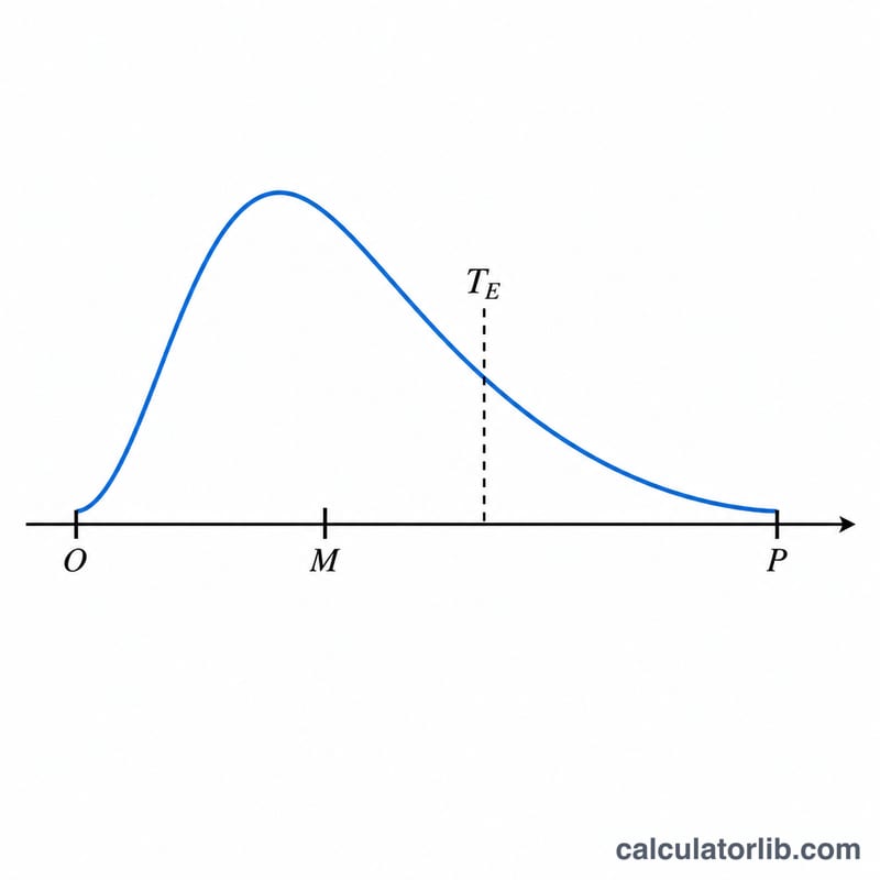
The PERT (Program Evaluation and Review Technique) calculator turns three time guesses into a single, statistically-weighted estimate. Instead of relying on one number, you provide an Optimistic (O), Most Likely (M), and Pessimistic (P) duration. The tool returns the Expected Time (TE), the Standard Deviation (SD), and the Variance — giving you both a realistic estimate and a measure of its uncertainty. It works for any unit of time (hours, days, weeks) as long as you stay consistent.
How to Use It
Enter your three estimates for a task. The Optimistic value is the best-case duration if everything goes smoothly, the Most Likely is your realistic call, and the Pessimistic is the worst-case scenario. Press calculate to see the weighted expected time and how much it might vary.
The Formula Explained
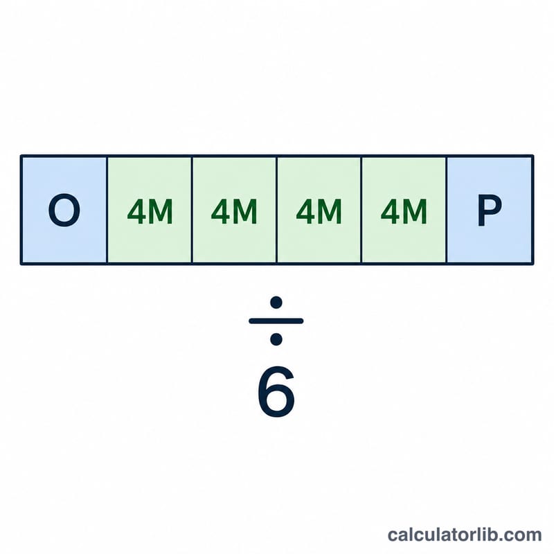
PERT uses a beta distribution and weights the most likely estimate four times more heavily than the extremes:
$$TE = \frac{\text{Optimistic (O)} + 4 \times \text{Most Likely (M)} + \text{Pessimistic (P)}}{6}$$
The spread of possible outcomes is captured by the standard deviation:
$$SD = \frac{\text{Pessimistic (P)} - \text{Optimistic (O)}}{6}$$
Variance is simply \(SD^{2}\). A large standard deviation signals a risky task that deserves a buffer.
Worked Example
Suppose a feature takes 4 days optimistically, 7 days most likely, and 16 days pessimistically. Then $$TE = \frac{4 + 4 \times 7 + 16}{6} = \frac{4 + 28 + 16}{6} = \frac{48}{6} = 8 \text{ days}.$$ $$SD = \frac{16 - 4}{6} = \frac{12}{6} = 2 \text{ days},$$ so variance \(= 4\). You would plan for 8 days, knowing roughly ±2 days of uncertainty.
Interpreting Your PERT Result
The expected time \(TE = \frac{O + 4M + P}{6}\) is the mean of a beta distribution that PERT uses to approximate the uncertain duration of a task. Once many tasks are added up, the total is roughly normal. Under that normal approximation, TE is the midpoint, so there is about a 50% chance of finishing by TE and about a 50% chance of taking longer. A TE on its own is therefore not a safe commitment date.
The standard deviation is approximated as \(SD = \frac{P - O}{6}\), and the variance is \(SD^2\). Under a normal approximation the SD gives these ranges:
- TE ± 1 SD covers about 68% of outcomes.
- TE ± 2 SD covers about 95%.
- TE ± 3 SD covers about 99.7%.
Example: O = 4, M = 7, P = 16 days gives \(TE = \frac{4 + 4 \times 7 + 16}{6} = \frac{48}{6} =\) 8 days, and \(SD = \frac{16 - 4}{6} = 2\) days.
- 68% range: 8 ± 2 = 6 to 10 days.
- 95% range: 8 ± 4 = 4 to 12 days.
- 99.7% range: 8 ± 6 = 2 to 14 days. Here the lower end is below the optimistic estimate of 4, which shows the normal approximation is imperfect at the tails.
A wide gap between P and O means a larger SD and higher risk, so look closely at what could drive the pessimistic case. The \((P-O)/6\) formula is a rule-of-thumb approximation, not an exact property of the beta distribution. The output is also only as good as the inputs: biased or guessed O, M and P values produce a precise-looking but unreliable result.
Scenario Comparison: How Estimate Spread Changes the Result
The table compares four sets of estimates (in any consistent time unit). The last column is the simple average \((O+M+P)/3\), shown for contrast.
| Scenario | O | M | P | TE | SD | Variance | Simple average |
|---|---|---|---|---|---|---|---|
| Symmetric | 4 | 6 | 8 | 6 | 0.67 | 0.44 | 6 |
| Right-skewed | 4 | 7 | 16 | 8 | 2 | 4 | 9 |
| Tight | 9 | 10 | 11 | 10 | 0.33 | 0.11 | 10 |
| Very uncertain | 2 | 10 | 30 | 12 | 4.67 | 21.78 | 14 |
Example calculation for the very uncertain case: \(TE = \frac{2 + 4 \times 10 + 30}{6} = \frac{72}{6} = 12\) and \(SD = \frac{30 - 2}{6} = 4.67\).
- When the estimates are symmetric or tight, TE equals M and the simple average.
- A long pessimistic tail pulls TE above M (7 becomes 8, 10 becomes 12).
- The SD depends only on the spread P − O, so the very uncertain case has a much larger SD than the tight one even though M is the same, 10.
- PERT puts more weight on M than the simple average does, so it is less sensitive to extreme O or P values.
PERT Terms and Definitions
- Optimistic (O): the shortest realistic duration if almost everything goes well.
- Most Likely (M): the duration you would expect under normal conditions; the most probable single value (the mode).
- Pessimistic (P): the longest realistic duration if significant problems occur, excluding catastrophic events.
- Expected Time (TE): the weighted mean \(\frac{O + 4M + P}{6}\).
- Standard Deviation (SD): a measure of uncertainty, approximated as \(\frac{P - O}{6}\).
- Variance: the square of the standard deviation, \(\left(\frac{P - O}{6}\right)^2\). Variances of independent tasks on a path can be added; standard deviations cannot.
- Beta distribution: a flexible probability distribution defined on a bounded interval, which can be skewed. PERT uses it to model task durations between O and P.
- Three-point estimation: estimating a task with three values (O, M, P) instead of one, so uncertainty is captured explicitly.
- Critical path: the longest sequence of dependent tasks in a project network. It determines the minimum project duration, and a delay in any task on it delays the project.
- PERT vs. triangular average: the triangular distribution mean is \(\frac{O + M + P}{3}\), which weights all three values equally. PERT weights M four times as heavily as O or P, so it relies more on the most likely value.
FAQ
Why is M multiplied by 4? The beta distribution assumes the most likely value dominates, so it carries four-sixths of the weight while O and P share the rest.
What units should I use? Any consistent time unit — hours, days, or weeks. The output uses the same unit as your inputs.
How do I combine many tasks? Sum the TE values for the total expected duration, and sum the individual variances (not standard deviations) before taking the square root for the overall SD.