What this A/B test calculator does
The calculator covers the three questions behind every conversion-rate experiment. Plan a test tells you how many visitors each variant needs to detect a chosen lift and how many days that takes at your traffic. Fixed sample works the other way round: for the visitors you already have, it gives the power to detect your effect and the smallest effect you can detect at the target power. Analyze results takes conversions and visitors for A and B and returns the observed lift, a two-proportion z-test p-value with a confidence interval, and the Bayesian probability that B beats A, all computed exactly with no random simulation.
The page opens with example inputs: a 5% baseline, a 10% relative minimum detectable effect, α = 5% two-sided and 80% power. Replace them with your own numbers.
Sample size formula
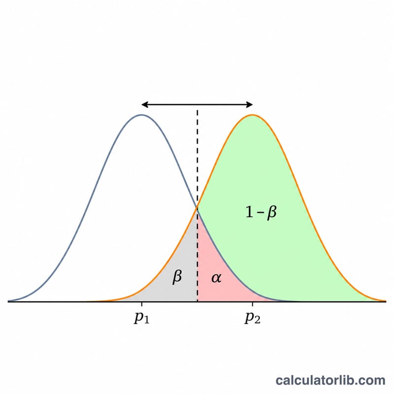
For two groups of equal size and conversion rates \( p_1 \) (control) and \( p_2 \) (variant), the visitors needed per group are
$$ n = \frac{\left( z_{1-\alpha/s}\sqrt{2\bar p(1-\bar p)} + z_{1-\beta}\sqrt{p_1(1-p_1)+p_2(1-p_2)} \right)^2}{(p_2-p_1)^2}, \qquad \bar p = \frac{p_1+p_2}{2} $$where \( s = 2 \) for a two-sided test and \( s = 1 \) for a one-sided test, and \( z \) is the standard normal quantile. This is equation 4.14 of Fleiss, Levin and Paik, Statistical Methods for Rates and Proportions (3rd ed., 2003): the standard deviation under the null hypothesis uses the pooled rate \( \bar p \), the one under the alternative uses each rate separately. It is the same normal approximation used by the pooled z-test you run at the end, so plan and analysis match. The result is rounded up to a whole visitor.
The table also shows the size with the continuity correction of Fleiss, Tytun and Ury (1980), \( n_{cc} = \frac{n}{4}\left(1+\sqrt{1+\frac{4}{n\,|p_2-p_1|} }\right)^2 \). Textbook tables often print this larger, more conservative number.
Worked examples you can check
Fleiss, Levin and Paik, page 74: \( p_1 = 0.60 \), \( p_2 = 0.70 \), α = 1% two-sided, power 95%. The formula gives 807.07, so 808 per group, and 827 with the continuity correction, the figure printed in the book. With 75% power it gives 479.6 (480), and 499.4 with the correction: the book prints 499, the calculator rounds up to 500. To reproduce it here, choose the absolute effect type with a baseline of 60 and an effect of 10.
Ryan (2013), as validated in the NCSS PASS manual: one-sided α = 5%, power 80%, 55% against 65% → 295.7, so 296 per group.
Default example: a 5% baseline and a 10% relative lift mean detecting 5.5% against 5%. With α = 5% two-sided and 80% power that needs 31,234 visitors per variant, 62,468 in total, or 32 days at 2,000 visitors a day.
Relative or absolute minimum detectable effect
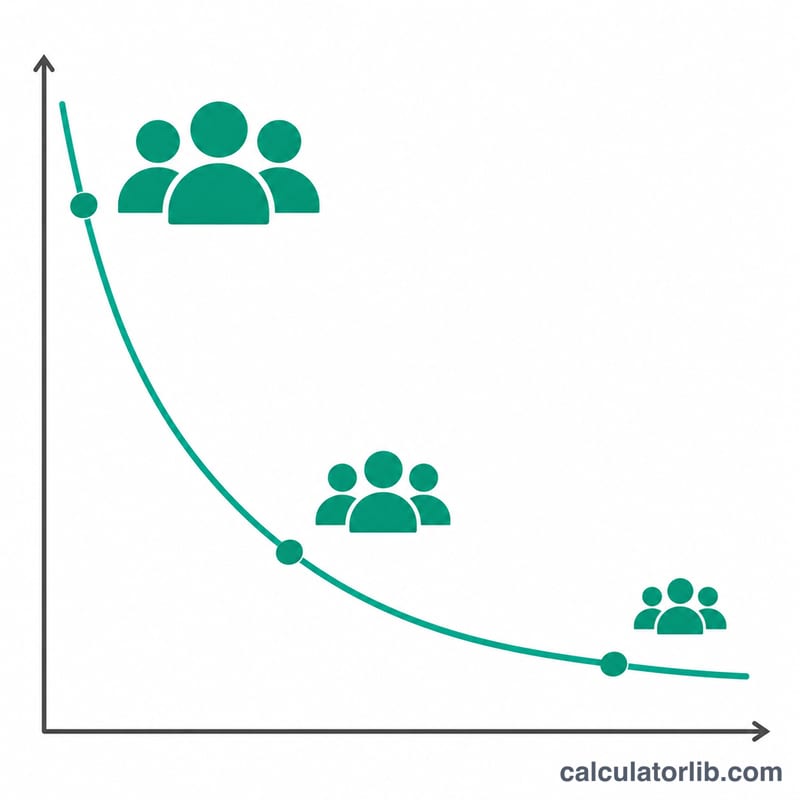
A relative effect of 10% on a 5% baseline means 5.5% (\( p_2 = p_1(1+\text{MDE}) \)). An absolute effect of 1 percentage point means 6% (\( p_2 = p_1 + \text{MDE} \)). Halving the effect roughly quadruples the sample, because \( n \) grows with \( 1/(p_2-p_1)^2 \). Low baselines are expensive: the same relative lift on a 1% rate needs about five times the visitors needed on a 5% rate.
Several variants and the Bonferroni correction
With \( k \) variants including the control, each of the \( k-1 \) challengers is compared with the control and every group gets the same \( n \), so the total is \( k \cdot n \). Each extra comparison is another chance of a false winner. The Bonferroni correction (Dunn, 1961) tests each comparison at \( \alpha/(k-1) \), which keeps the chance of at least one false positive at or below \( \alpha \). It is conservative, and it raises \( n \) for every group.
Power and minimum detectable effect for a fixed sample
Solving the same equation for power gives
$$ 1-\beta = \Phi\!\left( \frac{|p_2-p_1|\sqrt{n} - z_{1-\alpha/s}\sqrt{2\bar p(1-\bar p)} }{\sqrt{p_1(1-p_1)+p_2(1-p_2)} } \right) $$The calculator evaluates it for your effect and then searches for the smallest lift whose power reaches your target. Use this mode when traffic is fixed, for example a campaign that runs two weeks whatever happens: if the detectable lift is far larger than any realistic change, the test cannot tell you much.
Reading the results: p-value and confidence interval
With \( x_A \) conversions out of \( n_A \) visitors and \( x_B \) out of \( n_B \), the pooled z statistic is \( z = (\hat p_B-\hat p_A)/\sqrt{\hat p(1-\hat p)(1/n_A+1/n_B)} \) with \( \hat p = (x_A+x_B)/(n_A+n_B) \). The two-sided p-value is \( 2(1-\Phi(|z|)) \); the one-sided one, for the hypothesis that B is better, is \( 1-\Phi(z) \). The confidence interval for the difference uses the unpooled standard error, \( (\hat p_B-\hat p_A) \pm z_{1-\alpha/2}\sqrt{\hat p_A(1-\hat p_A)/n_A+\hat p_B(1-\hat p_B)/n_B} \). Example: 500 of 10,000 against 560 of 10,000 gives z = 1.894 and p = 0.0583, so the 12% observed lift is not significant at 5%, and the 95% interval for B − A runs from −0.02 to +1.22 percentage points.
Bayesian probability that B beats A
With a uniform Beta(1, 1) prior, the posterior of a conversion rate after \( x \) conversions in \( n \) visitors is Beta(\( 1+x \), \( 1+n-x \)) (Gelman et al., Bayesian Data Analysis, 3rd ed., chapter 2). Because these parameters are whole numbers, the probability that B's rate is higher has an exact finite sum:
$$ P(p_B>p_A) = \sum_{i=0}^{\alpha_B-1} \frac{B(\alpha_A+i,\ \beta_A+\beta_B)}{(\beta_B+i)\,B(1+i,\ \beta_B)\,B(\alpha_A,\ \beta_A)} $$with \( \alpha = 1+x \), \( \beta = 1+n-x \) and \( B \) the beta function, as derived by Evan Miller. The calculator evaluates it in log space, so it does not depend on random draws and gives the same answer every time. The expected loss of shipping B, \( E[\max(p_A-p_B, 0)] \), comes from the same sum with shifted parameters: it is the conversion rate you should expect to give up if B is in fact worse. For the example above, P(B > A) = 97.08% and the expected loss of shipping B is 0.0036 percentage points. "97% likely to be better" and "not significant at 5%" answer different questions; neither one is a licence to stop a test early.
Why peeking breaks a fixed-horizon test
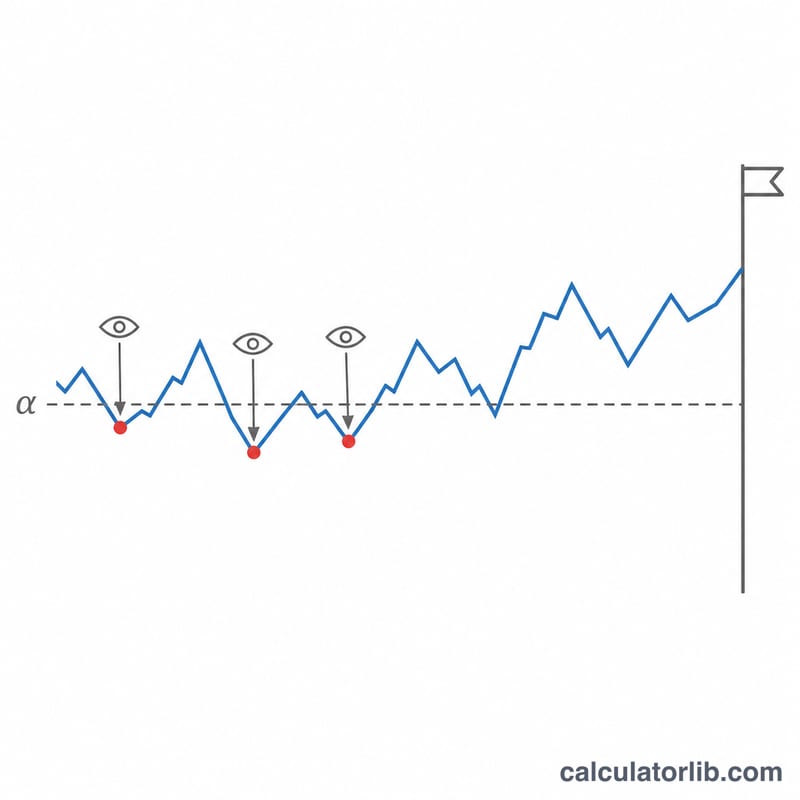
The sample size above assumes one look at the data, at the end. If you check after every batch and stop at the first p < 0.05, each look is another chance of a false positive. Armitage, McPherson and Rowe (1969) first measured this effect. Computed here by exact numerical integration of the joint normal distribution of the test statistics, for a 5% two-sided test with equally spaced looks and no real difference:
| Looks at the data | Chance of a false winner |
|---|---|
| 1 | 5.0% |
| 2 | 8.3% |
| 3 | 10.7% |
| 5 | 14.2% |
| 10 | 19.3% |
| 20 | 24.8% |
If you need to monitor a test while it runs, use a design built for it. Group-sequential boundaries such as O'Brien and Fleming (1979) spend very little α at the early looks and keep the overall false-positive rate at α. The alpha-spending approach of Lan and DeMets (1983) lets you look at times you did not fix in advance. Always-valid inference with the mixture sequential probability ratio test (mSPRT; Johari, Koomen, Pekelis and Walsh) gives p-values you may check at any moment. All of them need a larger maximum sample than a fixed-horizon test in exchange for that freedom.
Assumptions and limits
The formulas assume independent visitors, a stable conversion rate during the test and a fair random split. Run the test for whole weeks to cover day-of-week patterns, check that the traffic split matches the planned allocation, and count each visitor once. For very small samples or rates close to 0% or 100%, the normal approximation is rough; an exact test is safer there.
See also
Test already finished? The A/B test significance calculator checks whether the gap between two conversion rates is statistically significant, with the z-score and p-value.
Running a survey or poll? The sample size calculator tells you how many responses you need for a given confidence level and margin of error.