
What is cumulative binomial probability?
The cumulative binomial probability \(P(X \le k)\) gives the chance of obtaining at most k successes in n independent trials, where every trial has the same success probability p. It adds up the individual binomial probabilities from 0 successes all the way to k successes. This calculator is universal and applies to any binomial experiment such as coin flips, quality-control sampling, or pass/fail tests.
How to use the calculator
Enter three values: the number of trials (n), the number of successes you want the cutoff at (k), and the success probability per trial (p, a value between 0 and 1). The tool returns the cumulative probability \(P(X \le k)\) plus several related quantities: the exact probability \(P(X = k)\), the right-tail probabilities \(P(X > k)\) and \(P(X \ge k)\), and the distribution mean \(n \times p\).
The formula explained
Each term uses the binomial coefficient \(C(n,i) = \frac{n!}{i!\,(n-i)!}\), which counts how many ways i successes can occur, multiplied by \(p^i\) (the probability of those successes) and \((1-p)^{n-i}\) (the probability of the remaining failures). Summing these terms from \(i = 0\) to \(k\) yields the cumulative value:
$$P(X \le k) = \sum_{i=0}^{k} \binom{n}{i}\, p^{\,i}\,\left(1-p\right)^{n-i}$$To stay numerically stable for large n, the calculator builds each term from the previous one using the ratio \(\frac{n-i}{i+1} \times \frac{p}{1-p}\).
Worked example
Suppose you flip a fair coin 10 times (\(n = 10\), \(p = 0.5\)) and ask for the probability of at most 3 heads (\(k = 3\)). The four relevant terms are \(C(10,0)+C(10,1)+C(10,2)+C(10,3) = 1 + 10 + 45 + 120 = 176\), each multiplied by \(0.5^{10} = \frac{1}{1024}\). So $$P(X \le 3) = \frac{176}{1024} = 0.171875.$$
Interpreting Your Result
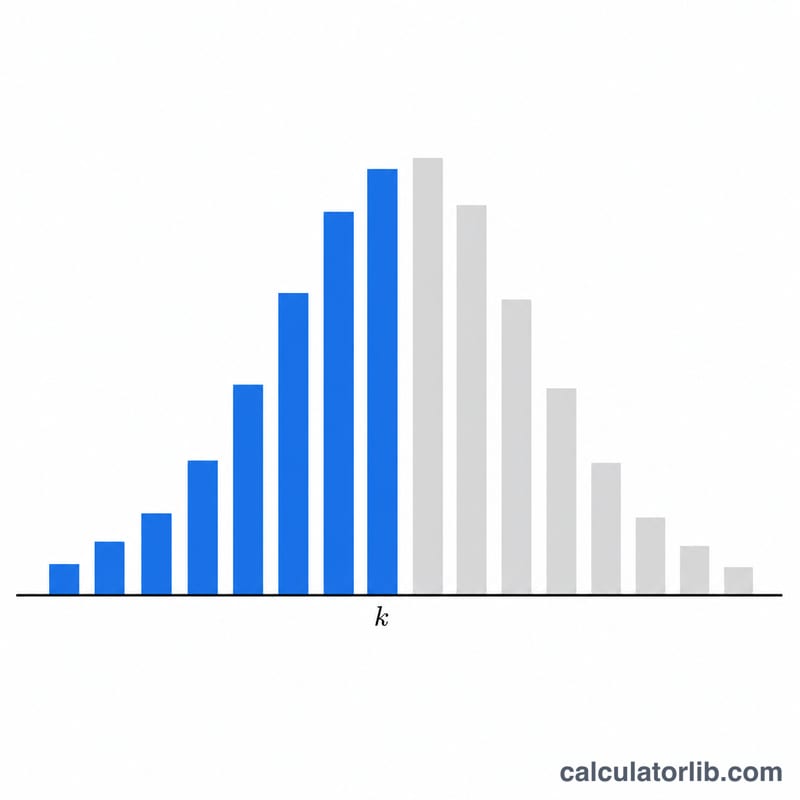
P(X ≤ k) is a cumulative probability. It answers "what is the chance of getting at most k successes?" by adding up the probabilities of 0, 1, 2, …, up to k successes. It is always between 0 and 1 and never decreases as k increases.
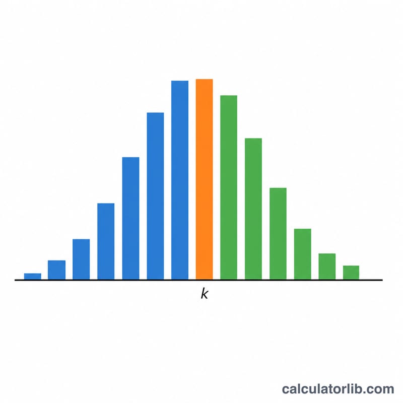
P(X = k) is a single point. It is the probability of exactly k successes — one term in the cumulative sum. So \(P(X\le k)\) is always at least as large as \(P(X=k)\), and \(P(X\le k)-P(X\le k-1)=P(X=k)\).
The two tails. The right tail \(P(X>k)=1-P(X\le k)\) is the chance of more than k successes, while \(P(X\ge k)=P(X>k)+P(X=k)\) includes k itself. Because the variable is a whole number of successes, \(P(X\ge k)=P(X\le k-1)\)'s complement is a common point of confusion — always check whether the cutoff value k should be counted in or out.
The mean. The expected number of successes is \(\mu = n\cdot p\). For n = 20 trials with p = 0.05 that is \(\mu = 1\) defective on average; for n = 10 with p = 0.9 it is \(\mu = 9\). Comparing your k to the mean tells you whether you are looking at a likely outcome (k near \(n\cdot p\)) or a tail event (k far from it).
Reading a number like 0.17. A result of \(P(X\le k)=0.17\) means there is a 17% chance of getting at most k successes — and therefore an 83% chance of getting more than k. Multiply by 100 to read it as a percentage.
When the right tail matters. Right-tail probabilities are central to decision thresholds and hypothesis testing. If you observe k successes and want to know how surprising that is under an assumed p, the upper-tail value \(P(X\ge k)\) acts as a one-sided p-value: a small value (commonly below 0.05) suggests the result is unlikely by chance alone. This is how acceptance-sampling plans set a maximum tolerable number of defects and how A/B tests flag unusually high success counts.
Definitions & Glossary
- n — number of trials. The fixed count of independent repetitions of the experiment (e.g. 20 inspected items, 10 coin flips).
- k — success cutoff. The number of successes of interest. In \(P(X\le k)\) it is the largest success count being included in the cumulative sum; \(k\) is a whole number from 0 to n.
- p — success probability. The chance of a "success" on a single trial, the same for every trial, with \(0\le p\le 1\).
- Success / failure. The two mutually exclusive outcomes of each trial. "Success" is simply the outcome you are counting; its complement, "failure," has probability \(1-p\).
- Binomial coefficient C(n, i). Written \(\binom{n}{i}=\dfrac{n!}{i!\,(n-i)!}\), it counts the number of distinct ways to arrange i successes among n trials.
- Cumulative probability. \(P(X\le k)=\sum_{i=0}^{k}\binom{n}{i}p^{i}(1-p)^{n-i}\), the total probability of k or fewer successes.
- Tail probability. The probability in one end of the distribution: the right (upper) tail \(P(X>k)=1-P(X\le k)\), or the inclusive upper tail \(P(X\ge k)\). Used for thresholds and p-values.
- Mean (expected value). \(\mu = n\cdot p\), the long-run average number of successes per n trials.
FAQ
What is the difference between \(P(X \le k)\) and \(P(X = k)\)? \(P(X = k)\) is the probability of exactly k successes, while \(P(X \le k)\) sums all outcomes from 0 up to and including k.
How do I get \(P(X \ge k)\)? Use the relationship \(P(X \ge k) = 1 - P(X \le k) + P(X = k)\), which this tool reports automatically.
Can p be 0 or 1? Yes. If \(p = 0\), you can never succeed so \(P(X \le k) = 1\) for any \(k \ge 0\); if \(p = 1\) all trials succeed.


