What this calculator does
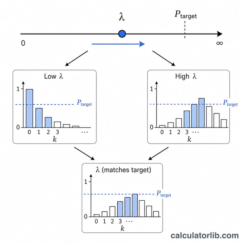
This tool is the inverse of the usual Poisson probability calculator. Instead of starting from a known mean lambda and computing a probability, you start from a known cumulative probability and a percentile point x, and the tool solves for the Poisson mean lambda that produces it. This is useful in capacity planning, reliability, and queueing when you know a target service level (a probability) and need the underlying expected rate of events.
How to use it
Choose a cumulative mode. Lower cumulative P means the probability you enter is P(X ≤ x), the chance of x or fewer events. Upper cumulative Q means it is Q(X ≥ x), the chance of x or more events. Enter the cumulative probability (a value strictly between 0 and 1) and the non-negative integer count x, then read off the mean lambda.
The formula explained
The Poisson mass function is \(f(t, \lambda) = e^{-\lambda} \lambda^{t} / t!\). The lower cumulative is the sum from \(t = 0\) to \(x\) and decreases as \(\lambda\) grows. The upper cumulative \(Q(x, \lambda) = 1 - P(x-1, \lambda)\) increases with \(\lambda\) for \(x \ge 1\). Because each cumulative is strictly monotonic in \(\lambda\), there is a unique solution, which the calculator finds with a robust bisection root finder evaluated by stable iterative term multiplication (no factorial overflow).
$$\sum_{k=0}^{x} \frac{\lambda^{k}\,e^{-\lambda}}{k!} = P$$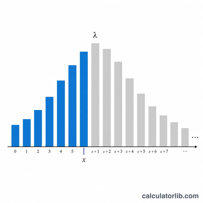
Worked example
Lower mode, \(P = 0.6\), \(x = 5\). We solve the sum of the first six Poisson terms equal to \(0.6\). Testing \(\lambda = 5.0\) gives \(P \approx 0.616\) (too high), \(\lambda = 5.1\) gives about \(0.597\), and \(\lambda = 5.08\) gives about \(0.600\). So \(\lambda\) is about \(5.083\) expected events.
FAQ
Why must the probability be strictly between 0 and 1? A probability of exactly 0 or 1 pushes lambda to a boundary (0 or infinity), so no finite unique mean exists.
What happens in upper mode with x = 0? \(Q(0, \lambda)\) is always 1 for every \(\lambda\), so the mean is undefined; the tool returns 0 for this degenerate case.
Does x have to be an integer? Yes, for the standard Poisson interpretation x is a non-negative integer count; non-integers are truncated.


