What this calculator does
This tool tabulates the Kelvin functions of the first kind, \(\mathrm{ber}_v(x)\) and \(\mathrm{bei}_v(x)\), for a chosen order (degree) \(v\) across a sweep of x values. These functions are the real and imaginary parts of the Bessel function \(J_v\) evaluated on the rotated argument \(x\cdot e^{i3\pi/4}\), and they appear in problems involving alternating-current resistance (skin effect), heat conduction in cylinders, and other physics and engineering applications.
How to use it
Enter four values: the order v (commonly 0, 1, 2…), the first x value x initial value, the Increment added each row, and the Number of iterations (table rows). The defaults sweep x from −7 to +7 in steps of 0.2 (71 rows). The result is a table of x, \(\mathrm{ber}_v(x)\), \(\mathrm{bei}_v(x)\).
The formula explained
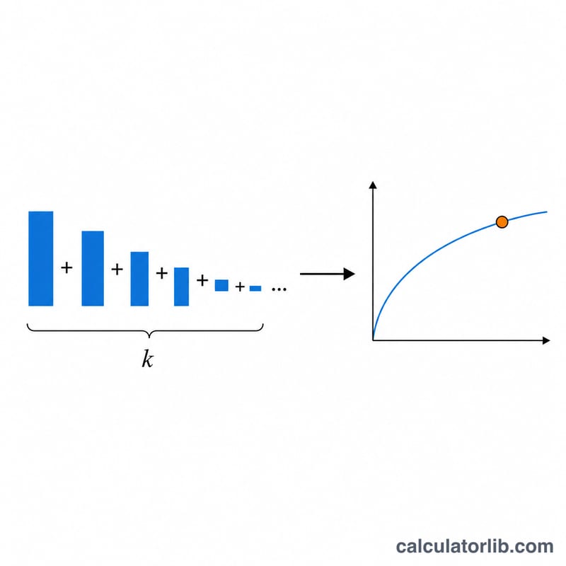
The series is $$\mathrm{ber}_v(x) + i\,\mathrm{bei}_v(x) = \left(\frac{x}{2}\right)^{v} e^{\,3v\pi i/4} \sum_{k=0}^{\infty} \frac{\left(\frac{i\,x^{2}}{4}\right)^{k}}{k!\,\Gamma(v+k+1)}$$ We evaluate it with complex term recurrence: each term equals the previous one multiplied by \(\frac{i\,x^{2}/4}{k(v+k)}\), which avoids recomputing powers and factorials. The Gamma function is computed via the Lanczos approximation for real \(v\). Summation stops when a term is negligible relative to the running sum.
Worked example (v = 0, x = 2)
The series give $$\mathrm{ber}_0(2) \approx 1 - 0.25 + 0.001736 - \dots \approx 0.75173$$ and $$\mathrm{bei}_0(2) \approx 1 - 0.027778 + 0.0000694 \approx 0.97229$$ matching standard tables (\(\mathrm{ber}_0(2)=0.7517\), \(\mathrm{bei}_0(2)=0.9723\)).
FAQ
Can v be non-integer? Yes. The Gamma function handles real \(v\). For negative x with non-integer \(v\) the prefactor \(\left(\frac{x}{2}\right)^{v}\) is multivalued; the principal branch is used.
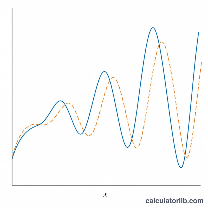
Why are values symmetric for v=0? The \(v=0\) series contains only even powers of x, so \(\mathrm{ber}_0(-x)=\mathrm{ber}_0(x)\) and \(\mathrm{bei}_0(-x)=\mathrm{bei}_0(x)\).
What about very large x? The series converges well for moderate \(|x|\). For \(|x| > 20\) many terms are needed and an asymptotic expansion would be more stable; keep within the default range for best accuracy.


