
What Is the Marginal Propensity to Consume?
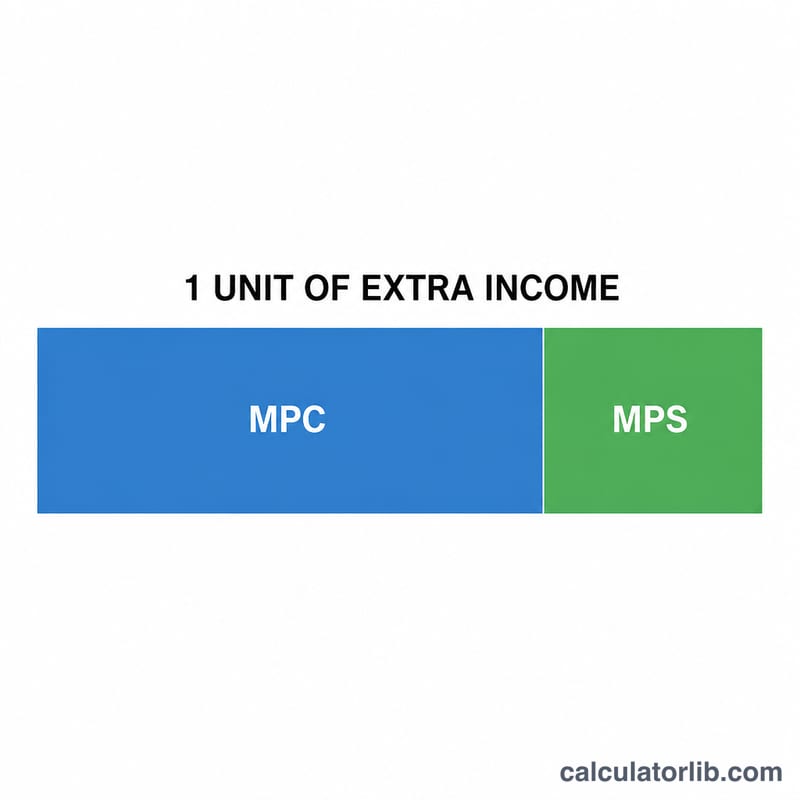
The Marginal Propensity to Consume (MPC) measures how much of each additional unit of income a household or economy spends rather than saves. It is one of the cornerstone concepts in Keynesian macroeconomics and a key driver of the fiscal multiplier. An MPC of 0.8 means that for every extra $1 earned, $0.80 is spent and $0.20 is saved.
How to Use This Calculator
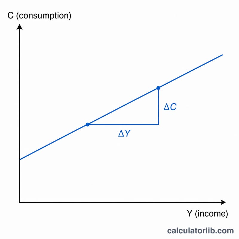
Enter the change in consumption (\(\Delta C\)) — how much spending increased — and the change in income (\(\Delta Y\)) — how much income increased. The calculator divides the two to give the MPC. It also reports the Marginal Propensity to Save (\(\text{MPS} = 1 - \text{MPC}\)) and the spending multiplier (\(1 \div \text{MPS}\)), which estimates how an initial injection of spending ripples through the economy.
The Formula Explained
$$\text{MPC} = \dfrac{\Delta C}{\Delta Y}$$ Because every extra dollar is either spent or saved, \(\text{MPC} + \text{MPS} = 1\), so \(\text{MPS} = 1 - \text{MPC}\). The multiplier follows from the geometric series of repeated spending rounds: $$k = \dfrac{1}{1 - \text{MPC}} = \dfrac{1}{\text{MPS}}$$ A higher MPC produces a larger multiplier.
Worked Example
Suppose income rises by $1,000 and consumption rises by $800. Then $$\text{MPC} = \frac{800}{1000} = 0.8$$ $$\text{MPS} = 1 - 0.8 = 0.2$$ and the multiplier $$= \frac{1}{0.2} = 5$$ A $100 boost in autonomous spending would therefore raise total output by about $500.
MPC Scenarios and Their Multipliers
In the simple Keynesian model, the MPS is \(1 - \text{MPC}\) and the spending multiplier is \(k = \frac{1}{1 - \text{MPC}} = \frac{1}{\text{MPS}}\). The table shows how the multiplier grows as households spend a larger share of each extra dollar. The last column shows the total change in output from an initial $100 spending injection (\(100 \times k\)).
| MPC | MPS (1 − MPC) | Multiplier (1/MPS) | Total output change from $100 injection |
|---|---|---|---|
| 0.50 | 0.50 | 2 | $200 |
| 0.60 | 0.40 | 2.5 | $250 |
| 0.75 | 0.25 | 4 | $400 |
| 0.80 | 0.20 | 5 | $500 |
| 0.90 | 0.10 | 10 | $1,000 |
| 0.95 | 0.05 | 20 | $2,000 |
Example: if MPC = 0.75, then MPS = 1 − 0.75 = 0.25 and \(k = 1 / 0.25 = 4\), so a $100 injection raises total output by \(4 \times \$100 = \$400\). These figures come from the simple textbook model, which ignores taxes, imports and other leakages.
Interpreting Your MPC Result
MPC is the share of each additional unit of income that is spent on consumption. Its complement, MPS, is the share saved. Together, \(\text{MPC} + \text{MPS} = 1\).
- Low MPC (below 0.5): Most extra income is saved. Spending responds weakly to income changes, so the simple multiplier is below 2 and an injection of spending has a limited knock-on effect.
- Moderate MPC (0.5 to 0.8): Income is split between spending and saving. The multiplier is between 2 and 5, which is typical of many textbook examples.
- High MPC (above 0.8): Most extra income is spent. The multiplier exceeds 5 and rises steeply as MPC approaches 1. Spending shocks are amplified strongly.
Boundary cases: If MPC = 0, all extra income is saved and the multiplier is \(1/(1-0) = 1\), meaning there is no knock-on effect. If MPC = 1, all extra income is spent, MPS = 0 and the multiplier \(1/0\) is undefined, or infinite in the simple model.
Unusual values: An MPC above 1 means consumption rose by more than income. This can reflect borrowing, drawing down savings, or a temporary effect. An MPC below 0 means consumption fell while income rose. Either result can also point to data problems, mismatched time periods, or one-off events. Check your inputs and the time period before relying on it.
Real-world caveat: The simple multiplier ignores taxes, imports, price changes and crowding out of private spending. Real-world multipliers are therefore usually smaller than \(1/(1-\text{MPC})\). This is general educational information, not personal financial advice.
Key Terms and Symbols
- Marginal Propensity to Consume (MPC)
- The fraction of an additional unit of income that is spent on consumption: \(\text{MPC} = \Delta C / \Delta Y\).
- Marginal Propensity to Save (MPS)
- The fraction of an additional unit of income that is saved: \(\text{MPS} = 1 - \text{MPC}\).
- Average Propensity to Consume (APC)
- Total consumption divided by total income (\(C/Y\)). It describes the overall spending share, not the share of an extra dollar.
- Change in consumption (ΔC)
- The change in spending on goods and services between two periods or scenarios.
- Change in income (ΔY)
- The change in income (usually disposable income) over the same periods or scenarios.
- Spending (fiscal) multiplier (k)
- The factor by which an initial change in spending changes total output. In the simple model, \(k = 1/(1-\text{MPC})\).
- Autonomous spending
- Spending that does not depend on current income, such as baseline consumption, some investment and government spending.
- Disposable income
- Income remaining after taxes (and net of transfers), available to spend or save.
FAQ
Can MPC be greater than 1? In theory MPC lies between 0 and 1, but short-term measurements can occasionally exceed 1 if households borrow to spend more than the income increase.
What is the difference between MPC and APC? MPC is the change in consumption per change in income (marginal), while the average propensity to consume (APC) is total consumption divided by total income.
Why does the multiplier matter? A larger MPC means money recirculates more, amplifying the effect of fiscal stimulus or any spending change on overall economic output.