What This Calculator Does
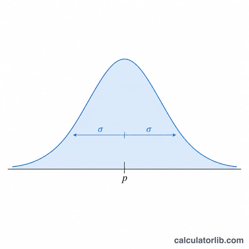
This tool describes the sampling distribution of the sample proportion (p̂). When you repeatedly draw random samples of size n from a population with true proportion p, the resulting sample proportions form their own distribution. This calculator returns its mean and standard error so you can build confidence intervals, run hypothesis tests, or assess sampling variability.
How to Use It
Enter the population proportion p as a decimal between 0 and 1 (for example, 0.4 for 40%), then enter the sample size n. The calculator instantly outputs the mean (which equals p), the variance, and the standard error (SE) of the sampling distribution.
The Formula Explained
The mean of the sampling distribution equals the population proportion: \(\mu_{\hat{p}} = p\). The standard error measures how much sample proportions vary around p and is given by $$\text{SE} = \sqrt{\frac{p(1-p)}{n}}$$ Larger samples shrink the standard error, making your estimate more precise. By the Central Limit Theorem, the distribution is approximately normal when both \(np \ge 10\) and \(n(1-p) \ge 10\).
Worked Example
Suppose \(p = 0.5\) and \(n = 100\). The mean is 0.5. The variance is $$0.5 \times 0.5 / 100 = 0.0025$$ and the standard error is $$\sqrt{0.0025} = 0.05$$ So sample proportions typically fall within about \(\pm 0.05\) of 0.5.
FAQ
Why does the mean equal p? Because the sample proportion is an unbiased estimator of the population proportion — on average it hits the true value.
What happens as n grows? The standard error decreases proportionally to \(1/\sqrt{n}\), so estimates become more precise with larger samples.
When is the normal approximation valid? A common rule is \(np \ge 10\) and \(n(1-p) \ge 10\); otherwise consider exact binomial methods.


