
What this calculator does
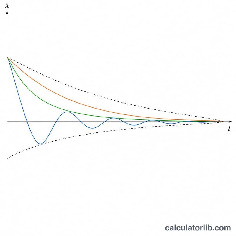
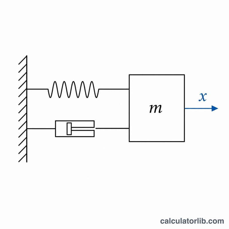
This tool computes the displacement \(x(t)\) of a one-dimensional damped harmonic oscillator that is released from rest at an initial displacement \(x_0\). It solves the standard mass-normalized equation of motion and tabulates the position over four natural periods, so you can see exactly how the system settles toward equilibrium. It also classifies the behavior as under-damped, critically damped, or over-damped.
The governing equation
The motion obeys the linear ordinary differential equation $$\frac{d^2x}{dt^2} + 2k\frac{dx}{dt} + \omega_0^2 x = 0,$$ where \(\omega_0\) is the undamped angular frequency and \(k\) is the resistance (damping) coefficient (both in units of \(1/s\)). With the initial conditions \(x(0) = x_0\) and \(\frac{dx}{dt}(0) = 0\), the closed-form solution depends on how \(k\) compares with \(\omega_0\).
When \(k < \omega_0\) the system is under-damped and oscillates with a reduced damped angular frequency $$\omega_d = \sqrt{\omega_0^2 - k^2},$$ the amplitude decaying as \(e^{-kt}\). When \(k = \omega_0\) the system is critically damped and returns to rest as fast as possible without oscillating: $$x(t) = x_0\left(1 + \omega_0\, t\right) e^{-\omega_0\, t}.$$ When \(k > \omega_0\) the system is over-damped and creeps back slowly with no oscillation.
How to use it
Enter the undamped angular frequency \(\omega_0\) (must be greater than zero), the damping coefficient \(k\) (zero or more, where \(k = 0\) gives pure undamped motion), the initial displacement \(x_0\), and the number of time divisions for the table. The natural period is \(T_0 = 2\pi/\omega_0\); the table spans \(4\,T_0\) in equal steps of \(dt = \text{timeSpan}/\text{divisions}\), giving \(\text{divisions}+1\) rows.
Worked example
For \(\omega_0 = 5\), \(k = 1\), \(x_0 = 1\) and 50 divisions the regime is under-damped with \(\omega_d = \sqrt{25 - 1} = 4.89898\) rad/s. The natural period is \(1.256637\) s, the span is \(5.026548\) s and \(dt = 0.100531\) s. At \(t = 0\) the displacement is 1; at the first step \(t = 0.100531\) s it is about \(0.884153\).
FAQ
What does the damping coefficient k represent? It is the mass-normalized half-damping term; the resistive force per unit mass equals \(2k\) times the velocity.
What if k equals w0 exactly? The under- and over-damped forms have a removable singularity there, so the tool uses the critical-damping formula whenever \(k\) is within a tiny tolerance of \(\omega_0\).
Why exactly four periods? Four natural periods is long enough to show the full decay envelope while keeping the table compact and readable.