What is the studentized range distribution?
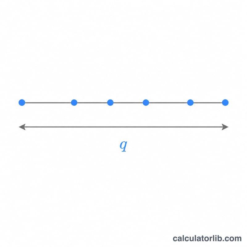
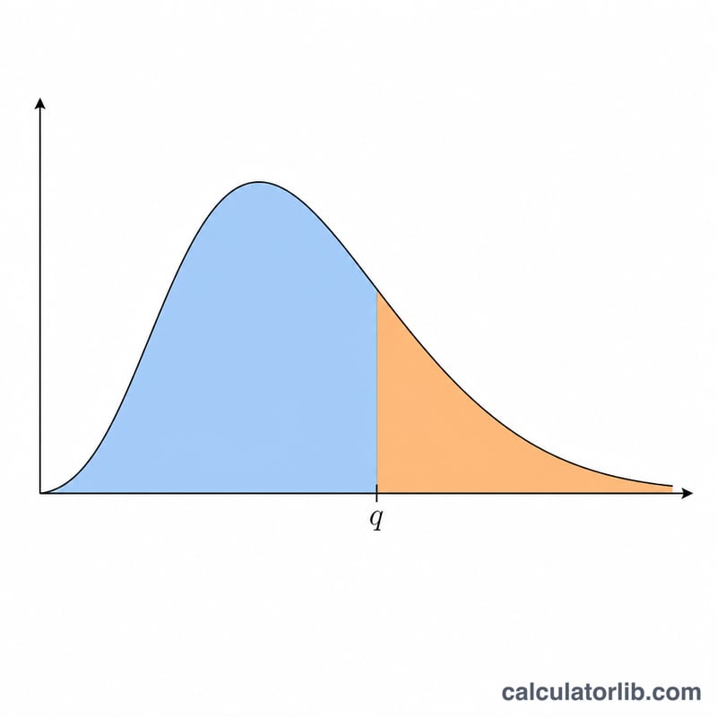
The studentized range statistic q measures the spread between the largest and smallest of r sample means, divided by an independently estimated standard error with nu degrees of freedom. Its distribution underlies Tukey's Honestly Significant Difference (HSD) test and other multiple-comparison post-hoc procedures. This calculator returns the lower cumulative probability \(P(Q \le q) = F(q, r, \nu)\) and the upper tail \(P(Q > q) = 1 - F\). It is a pure statistical function and applies universally, with no regional rules.
How to use it
Enter four numbers: the quantile q at which to evaluate the CDF, the sample size r (number of treatment means in the range, at least 2), the error degrees of freedom nu, and the number of independent groups c whose maximum range is taken (c = 1 is the ordinary studentized range; c > 1 models the maximum of c independent experiments sharing one critical value). The tool reports both tail probabilities.
The formula explained
For a fixed spread x, \(H(x, r)\) is the chance the range of r iid standard normals stays below x, computed as an integral of the standard normal density times \([\Phi(y) - \Phi(y - x)]\) raised to the power r-1. To account for the estimated variance, \(H(q\sqrt{u}, r)\) is averaged against the chi-square/nu scaling density of u (with nu degrees of freedom) and raised to the power c. When nu is extremely large the variance is known, the scaling collapses to u = 1, and the full expression $$F(q;r,\nu) = \int_{0}^{\infty} \frac{\nu^{\nu/2}}{\Gamma(\nu/2)\,2^{\nu/2-1}}\, u^{\nu-1} e^{-\nu u^2/2}\,\big[H(qu,\,r)\big]^{c}\,du$$ reduces to $$F = \big[H(q, r)\big]^{c}.$$
Worked example
With \(q = 5.673\), \(r = 5\), \(\nu = 5\), \(c = 1\) the calculator returns a lower cumulative probability of about 0.95, so the upper tail is about 0.05. This matches the classic Tukey q-table critical value of roughly 5.67 for five groups and five error degrees of freedom at \(\alpha = 0.05\).
FAQ
Why does my answer differ slightly from a printed table? The probability is found by numerical integration; accuracy degrades when r is large and nu is small, as the source method notes.
What does c do? \(c > 1\) gives the distribution of the maximum of c independent studentized ranges, useful when the same critical value is reused across c independent experiments.
What if q is zero or negative? A range cannot be negative, so \(F = 0\) and the upper probability is 1.


