What this calculator does
The Present Value of Annuity Calculator tells you how much a series of future payments is worth today. It handles every common variation in one engine: ordinary annuities (payments at the end of each interval), annuities due (payments at the start), growing annuities (each payment larger than the last), multiple payments per period, and arbitrary intra-period compounding. This is a universal financial-math tool and is not tied to any country or tax rule.
How to use it
Enter the time horizon in periods (t), the nominal rate per period as a percent (R), how many times interest compounds per period (m), the payment amount (PMT), the percentage each payment grows (G, use 0 for a level annuity), the number of payments per period (q), and whether payments arrive at the end (ordinary) or start (due). The calculator returns the present value, the effective discount rate per payment, and the total number of payments.
The formula explained
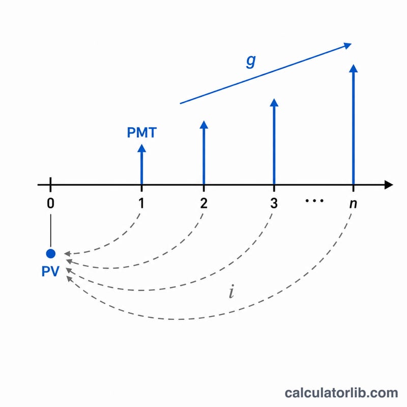
First the nominal rate is converted to an effective rate per payment interval: $$i = \left(1 + \frac{R}{m}\right)^{m/q} - 1$$ The total number of payments is \(n = q \times t\). The level-annuity present value is \(\frac{PMT}{i}\left(1 - (1+i)^{-n}\right)\); for a growing annuity it becomes $$PV = \frac{PMT}{i-g}\left(1 - \left(\frac{1+g}{1+i}\right)^{n}\right)$$ Multiplying by \((1 + i \times T)\) converts an ordinary result into an annuity due. Edge cases are handled cleanly: when \(i = 0\) the value is simply \(PMT \times n\), and when \(i = g\) the growing formula collapses to \(\frac{PMT \times n}{1+i}\), avoiding division by zero.
Worked example
Suppose t = 10, R = 5.25%, m = 12, PMT = $1,000, G = 3%, q = 12, payments at end. Then \(n = 120\), \(i = \left(1 + \frac{0.0525}{12}\right)^{12/12} - 1 = 0.004375\), and \(g = 0.03\). $$PV = \frac{1000}{0.004375 - 0.03}\left(1 - \left(\frac{1.03}{1.004375}\right)^{120}\right) \approx \$763{,}199.88$$ Because payments grow faster than they are discounted, the stream is worth far more than 120 level $1,000 payments.
FAQ
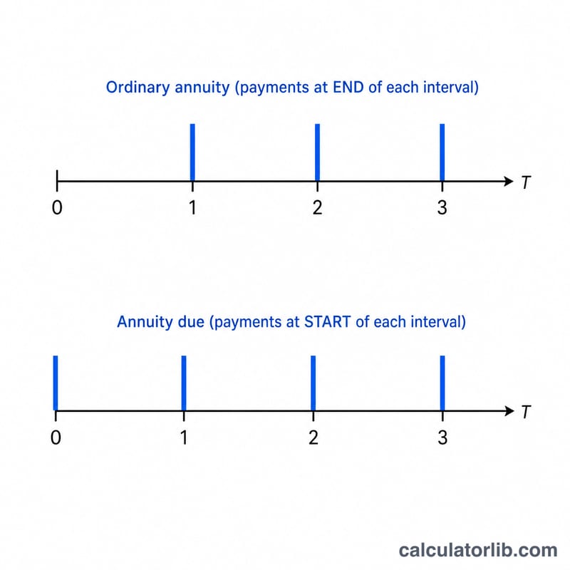
What is the difference between an ordinary annuity and an annuity due? An ordinary annuity pays at the end of each interval; an annuity due pays at the start, so each payment is discounted one interval less, making it worth \((1 + i)\) times more.
What does the growth rate do? It increases every successive payment by G percent, modeling raises, inflation-linked income, or escalating leases.
Can it model continuous compounding? Yes, in the limit: as m grows large, \(\left(1 + \frac{R}{m}\right)^{m}\) approaches \(e^{R}\), so a very large m closely approximates continuous compounding.