What is the Levy distribution?
The Levy distribution is a continuous probability distribution for a non-negative random variable. It is one of the few stable distributions that has a closed-form probability density, and it is also a special case of the inverse-gamma distribution. The distribution is described by two parameters: a location parameter mu, which shifts the distribution so its support begins at \(x = \mu\), and a scale parameter \(c > 0\), which controls the spread. Because of its very heavy right tail, the Levy distribution has an undefined (infinite) mean and variance, yet its pointwise density and cumulative probabilities are perfectly well defined.
How to use this calculator
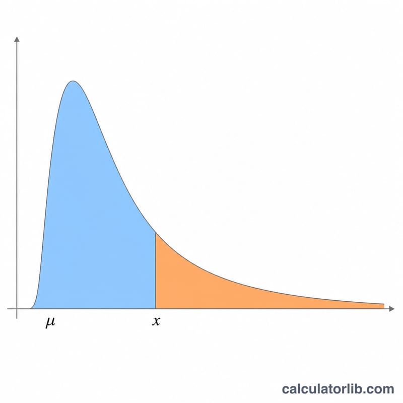
Enter the value of the random variable x, the location parameter mu, and the positive scale parameter c. The calculator returns the probability density \(f(x)\), the lower cumulative probability \(P(x) = P(X \le x)\), and the upper cumulative probability \(Q(x) = P(X > x)\). For the standard Levy distribution use \(\mu = 0\) and \(c = 1\). If x is at or below mu the variable lies outside the support, so the density is 0, \(P(x) = 0\) and \(Q(x) = 1\).
The formula explained
Let \(y = x - \mu\). For \(y > 0\) the density is $$f(x) = \sqrt{\dfrac{c}{2\pi}}\;\frac{e^{-\frac{c}{2y}}}{y^{3/2}}.$$ The cumulative distribution uses the complementary error function: $$P(x) = \operatorname{erfc}\!\left(\sqrt{\dfrac{c}{2y}}\right),$$ and the upper tail is simply $$Q(x) = 1 - P(x) = \operatorname{erf}\!\left(\sqrt{\dfrac{c}{2y}}\right).$$ This tool evaluates erf and erfc with the Abramowitz & Stegun rational approximation 7.1.26, which is accurate to about seven decimal places.
Worked example
Take \(\mu = 0\), \(c = 1\), \(x = 3\), so \(y = 3\). The argument is \(z = \sqrt{1/6} = 0.408248\). The density is $$\sqrt{\dfrac{1}{2\pi}}\cdot\frac{e^{-1/6}}{3^{1.5}} = \frac{0.398942 \cdot 0.846482}{5.196152} \approx 0.06499.$$ The lower cumulative probability is \(P(3) = \operatorname{erfc}(0.408248) \approx 0.56373\), and the upper cumulative probability is \(Q(3) = \operatorname{erf}(0.408248) \approx 0.43627\). As expected, \(P + Q = 1\).
FAQ
What happens if c is zero or negative? The scale parameter must be strictly positive; the calculator returns an error for \(c \le 0\).
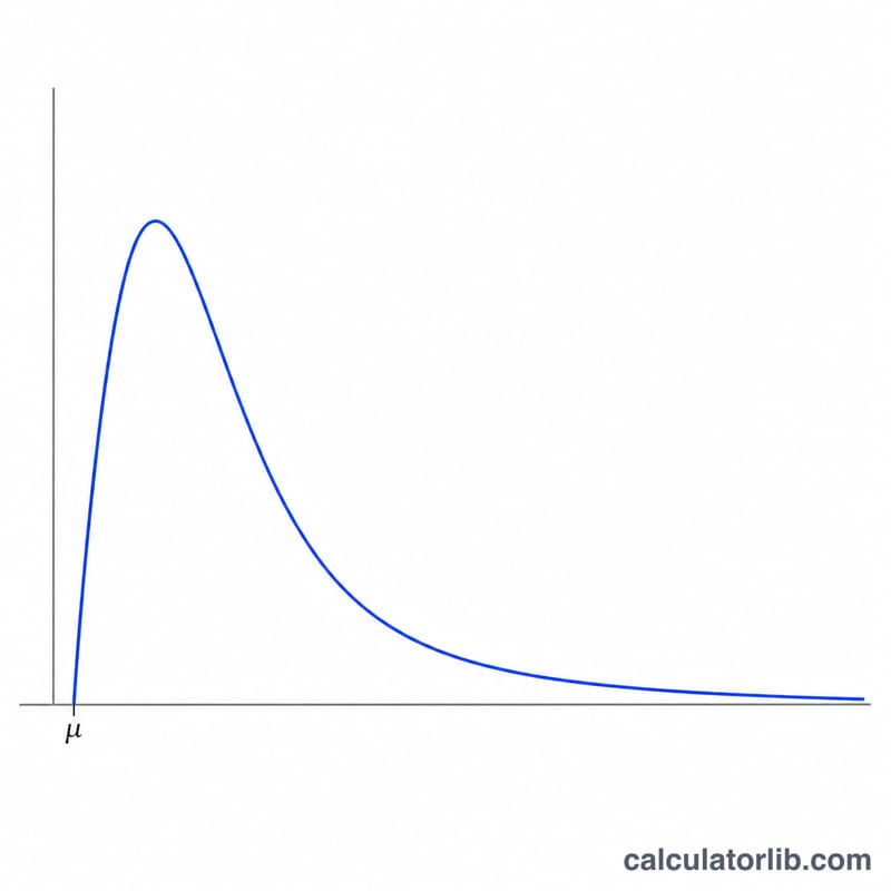
Why is the density 0 when x equals mu? The support starts at \(x = \mu\) and the density rises from 0, reaches a single mode, then decays slowly with a heavy right tail.
Does the Levy distribution have a mean? No. Both the mean and variance are infinite, which is why it is used to model phenomena with extreme outliers, such as Levy flights.


