What this calculator works out
It finds your break-even staying length: how many years you would have to live in a home before buying it costs less, on average per month, than renting a comparable place. It builds two 30-year cost paths — one where you buy, live, and sell at the end of year \(n\); one where you rent and invest the money you did not sink into a house — and reports the year the buying line drops below the renting line. You need it when a real offer and a real listing are in front of you and your horizon is uncertain: if you might move in three years, this is the whole decision.
How to read the inputs
Percentages go in as whole numbers (6.688 means 6.688%), and commas are fine in the dollar fields.
| Home purchase | Where it comes from | Sensible range |
|---|---|---|
| Home price | The accepted offer, not the list price | Any |
| Down payment | Cash you will actually wire, as % of price | 0–100 (100 = all cash) |
| Interest rate | Your locked rate | 0–10% |
| Loan term | Your mortgage term | 2 or more; blank means 30 |
| Buying closing costs | Lender, title and escrow fees, as % of price | 1–5% |
| Property tax | County rate, applied to the purchase price | 0.3–2.5%/yr |
| Property tax increase | Local assessment growth | 0–5%/yr |
| Home insurance | Annual premium quoted by your carrier | $800–$6,000 |
| HOA fee | Annual, from the listing (0 if none) | $0–$12,000 |
| Maintenance | % of home value per year | 1–2%/yr |
| Home value appreciation | Long-run local trend; may be negative | 0–5%/yr |
| Cost/insurance increase | Growth in premiums and HOA dues | 2–5%/yr |
| Selling closing costs | Agent commission plus transfer costs | 5–8% |
| Renting & you | Where it comes from | Sensible range |
|---|---|---|
| Monthly rental fee | Asking rent on the place you would take | Any |
| Rental fee increase | Market rent growth | 2–5%/yr |
| Renter's insurance | Per month, not per year | $10–$40 |
| Security deposit | Usually one month's rent; assumed refunded | $0–$6,000 |
| Upfront cost | Application and move-in fees — sunk | $0–$5,000 |
| Investment return | What the un-sunk cash would earn, before tax | 3–8%/yr |
| Federal / state marginal rate | Your top bracket on ordinary income | 0–50% combined |
| Tax filing status | Sets the deduction and the sale exclusion | Five options |
The formula
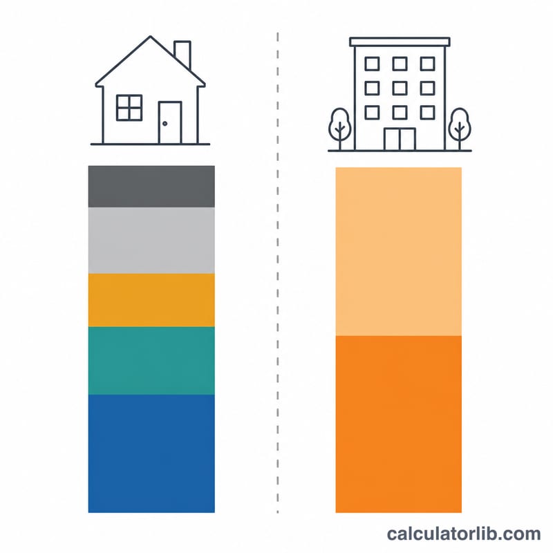
Let \(t\) be your combined marginal tax rate, \(r\) the investment return, and \(g\) the growth factor applied to every dollar tied up instead of invested:
$$g = 1 + r\,(1-t), \qquad t = t_{\text{federal}} + t_{\text{state}}$$Each year \(k\) produces one lump on each side — \(B_k\) for buying, \(R_k\) for renting:
$$B_k = \underbrace{12\,\text{pmt}}_{\text{only if } k\, \lt\, \text{term}} + T(1+i_T)^k + (I+H)(1+i_C)^k + \tfrac{m}{100}P(1+a)^k - t\cdot\max\!\left(0,\ \text{Int}_k + T_k - S\right)$$ $$R_k = 12\,(\text{rent} + \text{renter's insurance})\,(1+i_R)^k$$Here \(P\) = price, \(T\) = annual property tax, \(I\) = insurance, \(H\) = HOA, \(m\) = maintenance %, \(a\) = appreciation, \(S\) = standard deduction, and \(i_T, i_C, i_R\) are the three escalators. If you leave at the end of year \(n\), the totals in year-\(n\) dollars are
$$\text{Buy}(n) = U g^{n} + \sum_{k=1}^{n} B_k\,g^{\,n-k} - \left[V_n(1-c_s) - \text{balance}_n - \text{capgain tax}\right]$$ $$\text{Rent}(n) = (D + F)\,g^{n} - D + \sum_{k=1}^{n} R_k\,g^{\,n-k}$$with \(U\) = down payment plus buying closing costs, \(V_n\) = appreciated value, \(c_s\) = selling closing costs, \(D\) = deposit, \(F\) = upfront fee. Each total is divided by \(12n\) for the average monthly cost, and the break-even is where the two averages cross:
$$\text{break-even} = (n-1) + \frac{d_{n-1}}{d_{n-1} - d_n}, \qquad d_n = \text{buy}_n^{\text{monthly}} - \text{rent}_n^{\text{monthly}}$$A worked example
A $500,000 home, 20% down, 6.688% over 30 years, 2% buying and 7% selling closing costs, 1.5% property tax rising 3%/yr, $2,500 insurance, 1.5% maintenance, 3% appreciation; against $3,000/month rent rising 3%/yr with $15/month renter's insurance, a $3,000 deposit and $100 upfront; 5% investment return, 25% federal, married filing jointly.
$$g = 1 + 0.05\times(1-0.25) = 1.0375, \qquad \text{pmt} = \frac{400{,}000 \times 0.005573}{1-(1.005573)^{-360}} = \$2{,}577.93$$Year 1 of ownership, with the balance falling to $395,686.22 and the interest deduction taken as the average of the two year-end balances:
$$B_1 = 30{,}935.15 + 7{,}725.00 + 2{,}575.00 + 7{,}725.00 - 0.25\times(26{,}607.75 + 7{,}725 - 32{,}200) = \$48{,}426.96$$Sell at the end of year 1 for \(500{,}000\times1.03 = \$515{,}000\), netting $478,950 after the 7% selling cost — no gain tax, since that is below the basis. Proceeds are \(478{,}950 - 395{,}686.22 = \$83{,}263.78\), so
$$\text{Buy}(1) = 110{,}000 \times 1.0375 + 48{,}426.96 - 83{,}263.78 = \$79{,}288 \;\Rightarrow\; \$6{,}607/\text{month}$$ $$\text{Rent}(1) = 3{,}100 \times 1.0375 - 3{,}000 + 12\times3{,}015\times1.03 = \$37{,}482 \;\Rightarrow\; \$3{,}123/\text{month}$$Run the same loop further out: at year 7 the averages are $3,881 buying against $3,802 renting (buying $79/month dearer); at year 8, $3,905 against $3,930 (buying $25/month cheaper). Interpolating:
$$\text{break-even} = 7 + \frac{79}{79 - (-25)} = 7 + \frac{79}{104} = \mathbf{7.8\ \text{years}}$$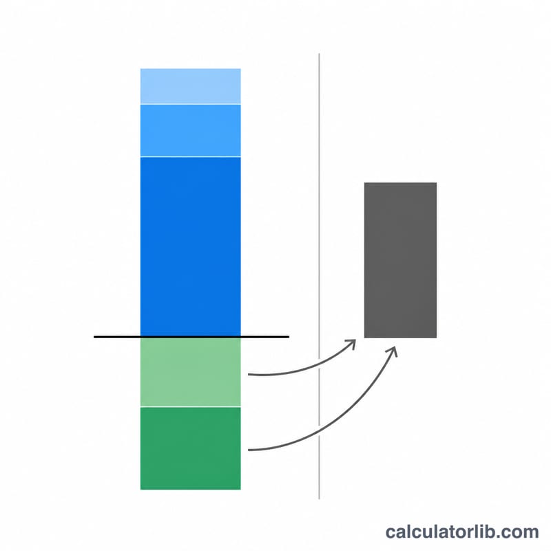
The rules that surprise people
Every recurring cost is already escalated in year 1. Property tax at 1.5% of $500,000 is charged as $7,725 in the first year, not $7,500 — each item grows a full year before it is ever billed.
Maintenance follows the home's value, not the price you paid. At 1.5% with 3% appreciation it climbs from $7,725 in year 1 to $18,204 in year 30. HOA dues ride the insurance escalator and renter's insurance rides the rent escalator; neither has one of its own.
The year your loan matures is free. Instalments are charged for the years before the term ends; in the final year the balance is simply cleared, with no payments and no interest deduction. On a 5-year term the average buying cost drops from about $43,500 to $22,000 between years 4 and 5, which flatters short terms.
Your tax rate quietly changes the investment return. Federal and state rates are added together, and the sum both prices the itemised deduction and haircuts the return: 5% at a 25% rate is applied as 3.75%. Raising your tax rate can move the break-even by nearly a year even when you claim no deduction.
The tax rules follow 2026 US law, simplified and held flat. The standard deduction is the 2026 IRS amount for your filing status — $16,100 single or married filing separately, $32,200 married filing jointly or qualifying surviving spouse, $24,150 head of household — and it is not inflated in later years. Mortgage interest counts only on the first $750,000 of the average loan balance ($375,000 if married filing separately), pro rata, and there is no SALT cap. Sale gains above the home-sale exclusion — $500,000 married filing jointly, $250,000 single, head of household or separately — are taxed at a flat 15%, the most common long-term capital-gains rate, not at your own bracket. A qualifying surviving spouse gets the $500,000 exclusion on the assumption that the home is sold within two years of the spouse's death. Sources: IRS Rev. Proc. 2025-32, IRC §121 (IRS Publication 523), IRC §163(h)(3)(F) (IRS Publication 936).
The comparison assumes you sell. Every row nets out that year's sale proceeds, after selling costs and the loan balance — which is why buying can show a negative average cost in a strong market, and why a higher selling cost pushes the break-even out.
The last crossing wins, not the first. With a short, expensive loan, buying can pull ahead the moment payments stop and then lose the lead again as taxes and maintenance compound. The year reported is the final crossing inside 30 years, sometimes a decade after the first.
"Renting is cheaper in the next 30 years" can appear when buying wins on every row. That message means no crossing was found — and if buying is ahead from day zero onward, there is nothing to cross. Zero out both closing-cost percentages and you will see it; read the table, not the sentence.
Loan term is fussy. Blank or 0 means 30 years; anything between 0 and 2 is rejected rather than corrected. Fractions such as 2.4 are accepted.
What Your Break-Even Year Actually Tells You
The break-even year \(t^{\ast}\) is the first year in the 30-year projection at which the cumulative cost of owning stops being higher than the cumulative cost of renting. If the calculator returns 9 years, it means that under the exact inputs you entered, buying and selling at the end of year 8 would have cost you more in total than renting the same period — and only from year 9 onward does ownership come out ahead. Nothing about the result says buying is "better"; it says buying wins if and only if you stay at least that long.
Both columns are converted to an average monthly figure so they can be read side by side:
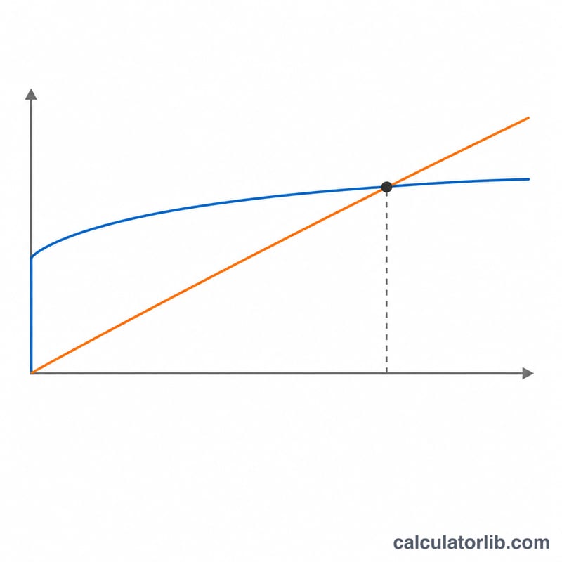
$$\text{Average monthly cost} = \frac{C(t)}{12\,t}$$Because the cumulative cost is divided by the months elapsed, the owning curve almost always starts very high (the down payment and buying closing costs are absorbed in year 1) and falls steeply, while the renting curve is comparatively flat and drifts upward with rent growth. The break-even year is simply where the falling curve crosses the drifting one.
Reading the three typical outcomes
- No break-even within 30 years. Owning never overtakes renting under your assumptions. This is normal, not an error. It usually appears when assumed appreciation is low relative to the assumed investment return, when the entered rent is low relative to the home price, when the interest rate is high, or when you enter a very large down payment (or an all-cash purchase) — a big lump of cash tied up in a home that appreciates at 3% loses to the same cash compounding at 6% in the renter's column, and 30 years is not long enough to close that gap.
- Break-even in year 1 or 2. Owning is cheaper almost immediately. This happens when rent is very high relative to the purchase price, when the mortgage rate is low, or when appreciation is set high enough that the equity gain at sale covers the upfront costs within a year or two. Treat single-digit-month break-evens with suspicion: they usually mean the rent figure, the appreciation figure, or both are optimistic.
- Break-even somewhere in years 5–12. The common middle case. It roughly matches the old rule of thumb that transaction costs (buying closing costs plus selling closing costs, often 8–10% of the price combined) need several years of amortization and appreciation to recover.
What the number is conditional on
The output is only as good as three forecasts you supplied and nobody can know: home value appreciation, rent growth, and the investment return applied to cash the renter does not sink into a down payment. Small changes in these move the break-even year by many years — see the scenario table below. Run the calculator two or three times with pessimistic and optimistic values and treat the result as a range, not a date.
Two mechanical assumptions also shape the answer. First, the sale is modeled at year-end of each year: selling closing costs are subtracted from the projected home value, the outstanding mortgage balance is repaid, and whatever is left is credited against the cost of owning. Second, the capital gain on that sale is tested against the primary-residence exclusion for the filing status you selected. That exclusion, along with the mortgage interest deduction, the standard deduction that limits it, and the state and local tax cap, are United States federal and state income tax rules — if you are outside the US, set the federal and state marginal rates to 0 and read the tax lines as not applicable, and substitute your own country's transfer taxes, stamp duty or capital gains treatment manually.
Finally, this is a cost comparison and nothing more. It cannot price the things that decide most real housing choices: the option to move for a job on 30 days' notice, security of tenure and freedom from landlord decisions, the ability to renovate, the risk of a forced sale in a down market, maintenance you do or don't want to be responsible for, and the discipline effect of a mortgage as forced saving. A calculator that says "buy after year 7" is silent on whether you will still want to live there in year 7. This section is general information, not financial, tax or legal advice; consult a qualified professional about your own situation.
How the Break-Even Year Shifts Across Scenarios
Every row below starts from one shared base case and changes exactly one lever, so the movement in the break-even year is attributable to that lever alone.
Base case: home price $450,000 · 20% down ($90,000) · 6.688% rate · 30-year term · 3% buying closing costs · 6% selling closing costs · 1.1% property tax rising 3%/yr · $1,800/yr home insurance · $0 HOA · 1% maintenance · cost/insurance inflation 3% · 3% appreciation · $2,400/mo rent rising 3%/yr · $15/mo renters insurance · $2,400 security deposit · $2,400 upfront rental cost · 6% investment return · married filing jointly · 24% federal + 5% state marginal rate.
The monthly payment behind every mortgaged row is
$$M = P\,\frac{i(1+i)^{n}}{(1+i)^{n}-1} = 360{,}000 \times \frac{0.00557333\,(1.00557333)^{360}}{(1.00557333)^{360}-1} \approx 2{,}320 \text{ per month}$$The figures below are what this calculator returns for each row under 2026 US tax rules, with the monthly averages rounded to the nearest $10; your own run will differ if any unlisted default differs.
| Scenario (one lever changed) | Changed input | Break-even | Buying: 10-yr avg monthly | Renting: 10-yr avg monthly | Direction of the effect |
|---|---|---|---|---|---|
| Base case | — | 7.5 years | ≈ $3,280 | ≈ $3,470 | Reference point: the buying and selling costs take most of eight years to recover. |
| Weak appreciation | homeValueAppreciationPct = 1 | 21.1 years | ≈ $4,070 | ≈ $3,470 | The single most powerful lever. Equity at sale collapses, so owning stays expensive far longer. |
| Strong appreciation | homeValueAppreciationPct = 5 | 3.1 years | ≈ $2,330 | ≈ $3,470 | Two extra points of appreciation on a $450,000 asset outweigh every other line item. |
| Fast rent inflation | rentalFeeIncreasePct = 5 | 5.7 years | ≈ $3,280 | ≈ $3,850 | Owning is unaffected; renting gets steadily worse, so the curves cross sooner. |
| Higher mortgage rate | interestRatePct = 7.5 | 11.6 years | ≈ $3,570 | ≈ $3,470 | More of each payment is interest, so principal (and equity) builds more slowly. |
| All-cash purchase | downPaymentPct = 100 | 3.1 years | ≈ $2,460 | ≈ $3,470 | With no loan there is no interest. The $463,500 tied up forgoes only about 4.26% a year after tax (6% × (1 − 0.29)), which is cheaper than borrowing at 6.688%. |
The remaining levers, in one line each
- rentalFeeIncreasePct = 2 — renting's 10-year average drops to roughly $3,300 and break-even slips to about 9.6 years. Rent-controlled or long-lease situations push buying out significantly.
- interestRatePct = 5 — buying's 10-year average falls to roughly $2,690 and break-even pulls in to about 3.8 years. Rate is the second-strongest lever after appreciation.
- downPaymentPct = 5 — the monthly payment rises to about $2,755 and break-even moves out to about 9.2 years: the extra interest on the bigger loan outweighs the smaller amount of cash tied up. Note this calculator has no PMI field; a low-down-payment loan in the US will normally carry mortgage insurance that the model does not charge you for, so treat this row as optimistic.
- investmentReturnPct = 4 — a lower return shrinks the opportunity cost on both sides (buying ≈ $2,850, renting ≈ $3,260), and break-even pulls in to about 5.9 years.
- investmentReturnPct = 8 — buying's 10-year average rises to roughly $3,750 against $3,700 for renting, and break-even stretches to about 10.9 years. Whether you assume 4% or 8% here moves the answer by about five years.
The pattern worth remembering: appreciation and investment return are assumptions, not facts, and they dominate the result. The mortgage interest deduction, by contrast, does nothing in this base case: about $23,900 of first-year interest plus about $5,100 of property tax comes to roughly $29,000, below the 2026 married-filing-jointly standard deduction of $32,200, and the gap only widens as the interest declines — so itemizing never beats the standard deduction here.
Key Terms Used in This Calculator
- Break-even staying length — the first year \(t\) at which cumulative owning cost no longer exceeds cumulative renting cost. Expressed in whole years because the model settles the sale at each year-end.
- Average monthly cost of owning — total cumulative cost of ownership through year \(t\), including upfront cash, divided by \(12t\). It is not your mortgage payment; it is an all-in figure net of sale proceeds, which is why it starts very high and falls each year.
- Opportunity cost / investment return — the return the money not spent on a down payment and closing costs could earn elsewhere. Entered as investmentReturnPct, it is credited to the renting column (the term \(G_t\) in the formula) and is one of the two assumptions that most strongly move the result.
- Buying closing costs — one-time fees paid at purchase (loan origination, appraisal, title, escrow, recording, transfer taxes). Entered as a percentage of the home price; commonly 2–5% in the US, but the specific fees and their names vary by country and by state.
- Selling closing costs — one-time costs at sale (agent commissions, transfer or conveyance taxes, legal fees). Entered as a percentage of the projected sale price and subtracted before net proceeds are computed. This is the main reason a short stay favors renting.
- PITI — the four components of a typical housing payment: Principal (the portion that reduces the loan balance), Interest (the lender's charge on the outstanding balance), Taxes (property tax) and Insurance (hazard/homeowner's insurance). Only principal builds equity; the other three are pure outflow.
- HOA fee — recurring dues to a homeowners' or condominium association covering shared maintenance, amenities and reserves. Entered here as an annual amount; it is a cost of owning that is never recovered at sale.
- Maintenance reserve — an annual allowance for repairs, replacements and upkeep, entered as a percentage of home value. A 1% assumption is a common planning convention; older homes and single-family houses typically run higher than newer condos, where part of the burden shifts into the HOA fee.
- Home value appreciation — the assumed compound annual growth rate of the property's market value. It drives both the equity credited at sale and (via the maintenance percentage) part of the ongoing cost. It is a forecast you supply, not a market fact.
- Mortgage interest deduction — a United States federal income tax provision allowing mortgage interest on a qualified residence to be deducted if you itemize. Its practical value here is only the amount by which your itemized deductions exceed the standard deduction, multiplied by your marginal rate — so for many borrowers with moderate loan balances the benefit is small or zero, and it shrinks every year as interest declines. Deductible state and local taxes, including property tax, are also subject to a statutory cap. This deduction does not exist in most other countries.
- Combined marginal tax rate — federal marginal rate plus state marginal rate, applied to the incremental deduction and, where relevant, to taxable gain. Marginal means the rate on your next dollar, not your average tax rate.
- Capital gain on sale and the primary-residence exclusion — the gain is broadly the net sale price minus your cost basis. Under US rules (IRC §121), a qualifying primary residence can exclude up to $250,000 of gain for a single filer, married filing separately, or head of household, and up to $500,000 for married filing jointly, provided ownership and use tests are met. The filing status you select determines which exclusion the model applies before taxing any excess.
- Amortization — the schedule by which a fixed payment is split between interest and principal. Early payments are mostly interest; the principal share grows over the term. This is why equity accumulates slowly in the first years and why a short stay rarely breaks even.
- Equity — current home value minus the outstanding loan balance. Net equity at sale (after selling closing costs and any tax on gain) is what the model subtracts from cumulative owning cost.
- Sunk cost vs refundable deposit — an upfront rental cost (application, broker or agency fee, first-month administrative charges) is non-recoverable and is added to the renting column permanently. A security deposit is, in principle, refundable at move-out and so is treated as returned cash rather than a cost. Deposit rules and caps are set by national or local law and differ widely.
These definitions are general information, not tax, legal or financial advice. Tax provisions named above are US-specific and change; confirm current rules and thresholds with a qualified professional before relying on them.
FAQ
Why does buying's average monthly cost fall and then climb again?
Early on, the large upfront cash is spread across more months, so the average drops. Later, the opportunity cost of everything tied up keeps compounding at \(g\) while the sale proceeds do not, so the average turns back up — at these inputs it bottoms at $3,881 in year 7 and reaches $6,283 by year 30.
Can the numbers come out negative?
Yes, and it is not an error. If appreciation and sale proceeds outrun the carrying costs, the average cost of buying is negative — the house paid you to live in it.
Does the security deposit count as a cost?
Only its opportunity cost. It is assumed returned in full, so a $12,000 deposit adds just $450 to first-year renting cost at a 3.75% after-tax return. The upfront fee, by contrast, is gone for good.
Why did a small rent change move my answer by a tenth of a year?
The crossing is searched on the whole-dollar monthly columns shown in the table, so a change that shifts one column by a dollar can tip the result to the next tenth. Treat the headline as good to about a tenth of a year.
Should I enter today's price or what I hope to sell for?
Today's price — the appreciation rate does the rest. It is worth running it twice, once at 0% appreciation and once at your local trend, to see how much of the answer rests on that one assumption.
See also: Rent or Buy Calculator — a simpler side-by-side comparison of the cost of renting and buying.